Week 3a: TerraTorch Foundations

Introduction

This session introduces foundation model workflows using TorchGeo and TerraTorch. You’ll learn to work with benchmark datasets, build production-ready models, and understand the fundamentals of geospatial deep learning with explicit PyTorch training loops.

Learning Objectives

By the end of this session, you will be able to:

Load benchmark datasets using TorchGeo
Build foundation models using TerraTorch’s EncoderDecoderFactory
Evaluate zero-shot performance and understand transfer learning
Implement few-shot learning with prototype networks
Use linear probing for efficient model adaptation
Train models using explicit PyTorch loops
Compare data efficiency across different training regimes

Why This Approach?

Traditional PyTorch training loops (see every step)
Manual metric calculation (understand the math)
Explicit device management (visible .to(device))
Debuggable workflows (inspect intermediate values)

Part 1: The TorchGeo/TerraTorch Ecosystem

The Library Stack

┌─────────────────────────────────────┐
│   Your Project Code                 │
├─────────────────────────────────────┤
│   TerraTorch (Model Factory)        │ ← Foundation models
├─────────────────────────────────────┤
│   TorchGeo (Dataset Handling)       │ ← Geospatial data
├─────────────────────────────────────┤
│   PyTorch (Deep Learning)           │ ← Core framework
└─────────────────────────────────────┘

TorchGeo provides:

Benchmark datasets (EuroSAT, BigEarthNet, etc.)
Geospatial data transforms
Samplers for efficient loading
Plotting and visualization utilities

TerraTorch provides:

Pre-trained foundation models (Prithvi, SatMAE, etc.)
Model factory for easy configuration
Encoder-decoder architectures
Task-specific heads

The EuroSAT Benchmark

EuroSAT is a land use classification dataset based on Sentinel-2 imagery.

Dataset Statistics:

Total images: ~27,000
Image size: 64×64 pixels
Bands: 13 (all Sentinel-2 bands)
Resolution: 10m, 20m, 60m (resampled to uniform grid)
Classes: 10 land use categories (original dataset)

Note: The TorchGeo version may have 9 classes. The code dynamically adapts to the actual number of classes in train_dataset.classes.

Typical Land Use Classes:

AnnualCrop
Forest
HerbaceousVegetation
Highway
Industrial
Pasture
PermanentCrop
Residential
River (may be merged with SeaLake in some versions)

Published Benchmarks:

ResNet-50: ~98% accuracy
VGG-16: ~97% accuracy
AlexNet: ~94% accuracy

Citation:

Helber, P., Bischke, B., Dengel, A., & Borth, D. (2019). EuroSAT: A novel dataset and deep learning benchmark for land use and land cover classification. IEEE Journal of Selected Topics in Applied Earth Observations and Remote Sensing, 12(7), 2217-2226.

Setup and Installation

import torch
import torch.nn as nn
from torch.utils.data import DataLoader
import numpy as np
import matplotlib.pyplot as plt
from pathlib import Path
import logging

logger = logging.getLogger(__name__)
# Set logging level to INFO
logger.setLevel(logging.INFO)

# Add handler for Jupyter notebook output
if not logger.handlers:
    handler = logging.StreamHandler()
    handler.setLevel(logging.INFO)
    formatter = logging.Formatter('%(message)s')
    handler.setFormatter(formatter)
    logger.addHandler(handler)

# Set random seeds for reproducibility
torch.manual_seed(42)
np.random.seed(42)

# Device selection
if torch.cuda.is_available():
    device = torch.device('cuda')
    logger.info(f"Using CUDA GPU: {torch.cuda.get_device_name(0)}")
elif torch.backends.mps.is_available():
    device = torch.device('mps')
    logger.info("Using Apple Silicon MPS")
else:
    device = torch.device('cpu')
    logger.info("Using CPU (training will be slower)")

logger.info(f"PyTorch version: {torch.__version__}")

Using Apple Silicon MPS
PyTorch version: 2.7.1

Part 2: Classification with EuroSAT

Step 1: Load the Dataset

TorchGeo makes loading benchmark datasets simple and standardized.

from torchgeo.datasets import EuroSAT

# Define data directory
data_dir = Path("data")
data_dir.mkdir(exist_ok=True)

# Load EuroSAT dataset with all bands
# First time will download ~90MB dataset
logger.info("Loading EuroSAT dataset...")
train_dataset = EuroSAT(
    root=str(data_dir),
    split="train",
    download=True
)

val_dataset = EuroSAT(
    root=str(data_dir),
    split="val",
    download=True
)

test_dataset = EuroSAT(
    root=str(data_dir),
    split="test",
    download=True
)

logger.info(f"Training samples: {len(train_dataset)}")
logger.info(f"Validation samples: {len(val_dataset)}")
logger.info(f"Test samples: {len(test_dataset)}")
logger.info(f"Number of classes: {len(train_dataset.classes)}")
logger.info(f"Classes: {train_dataset.classes}")

Loading EuroSAT dataset...
Training samples: 16200
Validation samples: 5400
Test samples: 5400
Number of classes: 10
Classes: ['AnnualCrop', 'Forest', 'HerbaceousVegetation', 'Highway', 'Industrial', 'Pasture', 'PermanentCrop', 'Residential', 'River', 'SeaLake']

Understanding the Dataset Object

The train_dataset is a PyTorch Dataset object with:

__len__() - Returns number of samples
__getitem__(idx) - Returns (image, label) tuple
.classes - List of class names
.split - Current split (train/val/test)

This standardization means the same code works for any TorchGeo dataset.

Step 2: Explore the Data

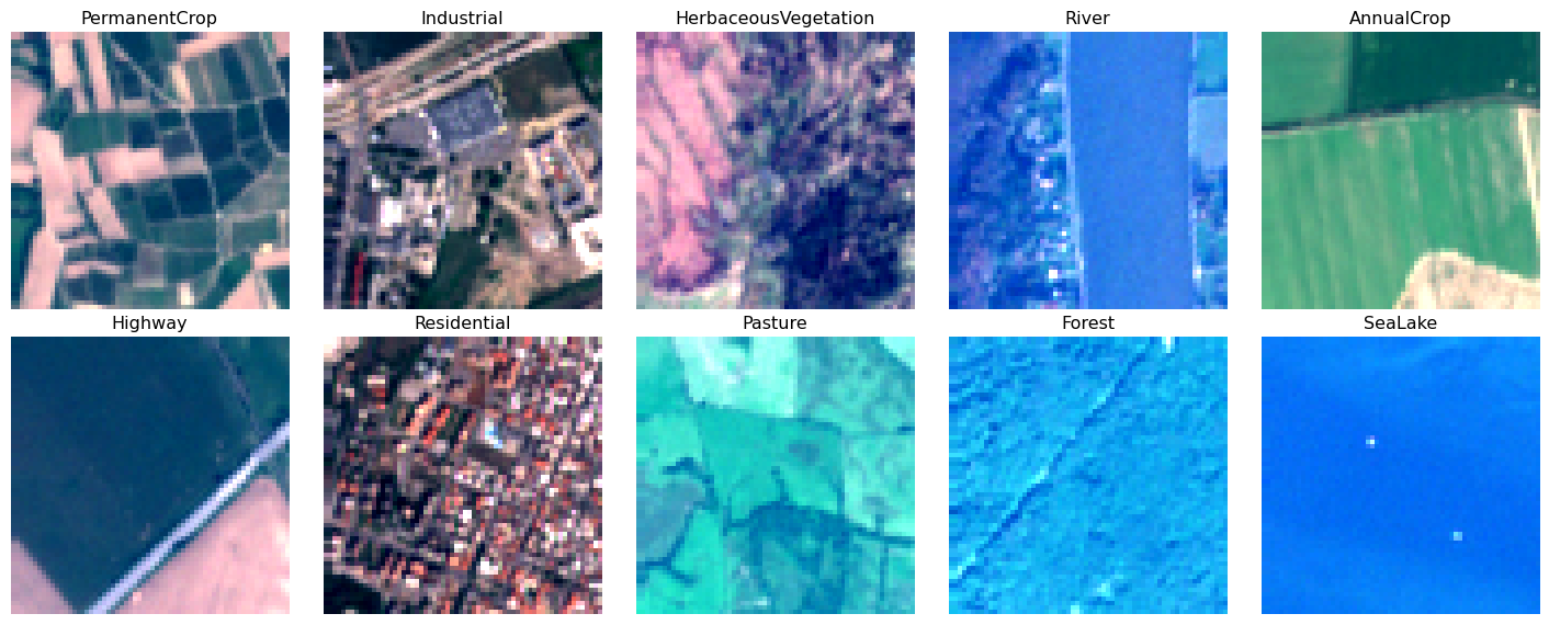
Let’s visualize samples from each class to understand what we’re working with.

# Get one sample from each class efficiently using random sampling
import random

samples_per_class = {}
num_classes = len(train_dataset.classes)
dataset_size = len(train_dataset)

# Random sampling is much faster than sequential scan
# Sample more indices than classes to ensure we find all classes quickly
random_indices = random.sample(range(dataset_size), min(dataset_size, num_classes * 10))

logger.info(f"Sampling representative images (one per class)...")
for idx in random_indices:
    sample = train_dataset[idx]
    image = sample["image"]
    label = sample["label"]
    class_idx = int(label) if hasattr(label, "item") else label

    if class_idx not in samples_per_class:
        samples_per_class[class_idx] = image

    # Stop once we have all classes
    if set(samples_per_class.keys()) == set(range(num_classes)):
        logger.info(f"Found all {num_classes} classes in {len(samples_per_class)} samples")
        break

# Create RGB composite for visualization
# EuroSAT bands: [B01, B02, B03, B04, B05, B06, B07, B08, B8A, B09, B10, B11, B12]
# RGB = B04 (Red), B03 (Green), B02 (Blue) = indices [3, 2, 1]

# Dynamic grid based on actual number of classes found
n_samples = len(samples_per_class)
n_cols = 5
n_rows = int(np.ceil(n_samples / n_cols))

fig, axes = plt.subplots(n_rows, n_cols, figsize=(15, 3*n_rows))
axes = axes.ravel()

for idx, (label, image) in enumerate(samples_per_class.items()):
    # Extract RGB bands
    rgb = image[[3, 2, 1], :, :].numpy()  # Red, Green, Blue
    rgb = np.transpose(rgb, (1, 2, 0))  # (H, W, C)

    # Normalize for display (using percentile stretch)
    p2, p98 = np.percentile(rgb, (2, 98))
    rgb_norm = np.clip((rgb - p2) / (p98 - p2), 0, 1)

    axes[idx].imshow(rgb_norm)
    axes[idx].set_title(train_dataset.classes[label])
    axes[idx].axis('off')

# Hide any unused subplots
for idx in range(n_samples, len(axes)):
    axes[idx].axis('off')

plt.tight_layout()
plt.show()

# Print band information and data range
logger.info(f"\nImage shape: {image.shape}")
logger.info(f"Bands: 13 Sentinel-2 bands")
logger.info(f"Spatial size: 64×64 pixels")
logger.info(f"")
logger.info(f"Raw EuroSAT data range:")
logger.info(f"  Min value: {image.min():.2f}")
logger.info(f"  Max value: {image.max():.2f}")
logger.info(f"  Mean value: {image.mean():.2f}")
logger.info(f"")
logger.info(f"This confirms EuroSAT is NOT pre-normalized!")
logger.info(f"Typical Sentinel-2 range: 0-10000 (surface reflectance × 10000)")

Sampling representative images (one per class)...
Found all 10 classes in 10 samples


Image shape: torch.Size([13, 64, 64])
Bands: 13 Sentinel-2 bands
Spatial size: 64×64 pixels

Raw EuroSAT data range:
  Min value: 5.00
  Max value: 1236.00
  Mean value: 337.57

This confirms EuroSAT is NOT pre-normalized!
Typical Sentinel-2 range: 0-10000 (surface reflectance × 10000)

Band Selection Strategy

Challenge: Prithvi expects 6 bands, EuroSAT has 13 bands.

Solution: Select the 6 bands Prithvi was trained on:

B02 (Blue) - 10m
B03 (Green) - 10m
B04 (Red) - 10m
B08 (NIR) - 10m
B11 (SWIR1) - 20m
B12 (SWIR2) - 20m

EuroSAT indices: [1, 2, 3, 7, 11, 12]

Step 3: Create Data Transforms

We need to select the correct bands and normalize the data for Prithvi.

Critical Understanding:

EuroSAT raw data: Sentinel-2 surface reflectance values (typically 0-10000+)
Prithvi expects: Normalized values in range [0, 1]
Why this matters: Without normalization, the model gets completely out-of-distribution inputs
Result without normalization: Zero-shot accuracy ~10% (random guessing)

import torch

def select_prithvi_bands(sample):
    """
    Select the 6 bands Prithvi was trained on from EuroSAT's 13 bands.

    Parameters
    ----------
    sample : dict
        TorchGeo sample with 'image' and 'label' keys

    Returns
    -------
    dict
        Sample with 6-band image
    """
    # EuroSAT band order: [B01, B02, B03, B04, B05, B06, B07, B08, B8A, B09, B10, B11, B12]
    # Prithvi bands: [B02, B03, B04, B08, B11, B12]
    # Indices: [1, 2, 3, 7, 11, 12]

    image = sample['image']
    selected_bands = image[[1, 2, 3, 7, 11, 12], :, :]

    return {
        'image': selected_bands,
        'label': sample['label']
    }

def normalize_prithvi(sample):
    """
    Normalize imagery for Prithvi using per-sample normalization.

    In production, you would want to use global statistics from the training set.
    For this demo, we use per-sample percentile normalization.

    Parameters
    ----------
    sample : dict
        Sample with 'image' and 'label'

    Returns
    -------
    dict
        Sample with normalized image
    """
    image = sample['image']

    # Normalize each band independently using 2nd-98th percentile
    normalized = torch.zeros_like(image)
    for c in range(image.shape[0]):
        band = image[c]
        p2, p98 = torch.quantile(band, torch.tensor([0.02, 0.98]))
        normalized[c] = torch.clamp((band - p2) / (p98 - p2 + 1e-8), 0, 1)

    return {
        'image': normalized,
        'label': sample['label']
    }

from torchvision import transforms

# Compose transforms
transform = transforms.Compose([
    select_prithvi_bands,
    normalize_prithvi  # Critical for Prithvi - expects [0, 1] normalized inputs
])

# Apply transforms to datasets
class TransformedDataset(torch.utils.data.Dataset):
    """Wrapper to apply transforms to TorchGeo datasets."""
    def __init__(self, dataset, transform=None):
        self.dataset = dataset
        self.transform = transform

    def __len__(self):
        return len(self.dataset)

    def __getitem__(self, idx):
        sample = self.dataset[idx]
        if self.transform:
            sample = self.transform(sample)
        return sample['image'], sample['label']

train_dataset_transformed = TransformedDataset(train_dataset, transform)
val_dataset_transformed = TransformedDataset(val_dataset, transform)
test_dataset_transformed = TransformedDataset(test_dataset, transform)

# Test the transformation
sample_img, sample_label = train_dataset_transformed[0]
logger.info(f"Transformed image shape: {sample_img.shape}")
logger.info(f"Expected: (6, 64, 64)")
logger.info(f"Label: {sample_label} ({train_dataset.classes[sample_label]})")
logger.info(f"Value range: [{sample_img.min():.4f}, {sample_img.max():.4f}]")
logger.info(f"Expected range: [0, 1] after normalization")

Transformed image shape: torch.Size([6, 64, 64])
Expected: (6, 64, 64)
Label: 0 (AnnualCrop)
Value range: [0.0000, 1.0000]
Expected range: [0, 1] after normalization

Step 4: Create DataLoaders

DataLoaders handle batching, shuffling, and parallel data loading.

# Create DataLoaders
train_loader = DataLoader(
    train_dataset_transformed,
    batch_size=32,
    shuffle=True,
    num_workers=0  # Set to 0 for Windows, 4+ for Linux/Mac
)

val_loader = DataLoader(
    val_dataset_transformed,
    batch_size=32,
    shuffle=False,
    num_workers=0
)

test_loader = DataLoader(
    test_dataset_transformed,
    batch_size=32,
    shuffle=False,
    num_workers=0
)

logger.info(f"Training batches: {len(train_loader)}")
logger.info(f"Validation batches: {len(val_loader)}")
logger.info(f"Test batches: {len(test_loader)}")

# Test a batch
images, labels = next(iter(train_loader))
logger.info(f"\nBatch shape: {images.shape}")
logger.info(f"Labels shape: {labels.shape}")
logger.info(f"Batch on device will be: {images.to(device).device}")

Training batches: 507
Validation batches: 169
Test batches: 169

Batch shape: torch.Size([32, 6, 64, 64])
Labels shape: torch.Size([32])
Batch on device will be: mps:0

Step 5: Build the Model

TerraTorch’s EncoderDecoderFactory makes it simple to build models. How build_model Works

The build_model method from EncoderDecoderFactory creates a flexible model by combining a backbone (encoder) with a task-specific decoder head. For classification, the decoder will produce logits of shape [batch_size, num_classes]. This method is highly customizable and is central to TerraTorch’s architectural flexibility.

Key arguments to build_model:

task: The type of task ("classification", "segmentation", "regression", etc.)
backbone: The encoder backbone to use (e.g., "prithvi_eo_v1_100", "prithvi_eo_v2_300", "satmae", "clay", "timm_resnet50")
decoder: The decoder architecture to attach. For classification, "FCNDecoder" is a typical choice; for segmentation, you might use "SegmentationDecoder" or others suitable for the task.
num_classes: The number of output classes for classification (or channels for other tasks)

Further arguments (advanced):

pretrained: If True, will use pretrained weights for the backbone where available.
in_channels: Number of input channels; must match your data (EuroSAT uses 6 bands).
freeze_encoder: If True, the backbone weights will not be updated during training.
decoder_kwargs: Dictionary of extra arguments for fine-tuning decoder behavior.

For official documentation and a full list of arguments, see:
https://terratorch.readthedocs.io/en/latest/api/terratorch.models.html#terratorch.models.EncoderDecoderFactory.build_model

from terratorch.models import EncoderDecoderFactory

# Create model factory
model_factory = EncoderDecoderFactory()

# Build classification model with Prithvi backbone
num_classes = len(train_dataset.classes)

model = model_factory.build_model(
    task="classification",
    backbone="prithvi_eo_v1_100",  # 100M parameter Prithvi
    decoder="FCNDecoder",           # Simple fully-convolutional decoder
    num_classes=num_classes         # Based on actual dataset
)

# Move model to device
model = model.to(device)

# Count parameters
total_params = sum(p.numel() for p in model.parameters())
trainable_params = sum(p.numel() for p in model.parameters() if p.requires_grad)

logger.info(f"Model loaded: Prithvi-100M with FCN decoder")
logger.info(f"Total parameters: {total_params:,}")
logger.info(f"Trainable parameters: {trainable_params:,}")
logger.info(f"Model on device: {next(model.parameters()).device}")

Model loaded: Prithvi-100M with FCN decoder
Total parameters: 90,176,010
Trainable parameters: 90,176,010
Model on device: mps:0

Understanding the Architecture

Encoder (Backbone):

prithvi_eo_v1_100 - Vision Transformer pretrained on HLS imagery
Extracts spatial features from 6-band input
Parameters frozen or fine-tuned depending on task

Decoder (Head):

FCNDecoder - Fully Convolutional Network
Aggregates encoder features
Produces class logits (num_classes outputs)

Alternative backbones: prithvi_eo_v2_300, satmae, scalemae, clay, timm_resnet50

Part 3: Zero-Shot Inference - Baseline Performance

Before training the model, let’s evaluate what the pretrained Prithvi backbone already knows. This establishes a baseline and demonstrates the power of transfer learning.

Understanding Zero-Shot Inference

Zero-shot inference means using a model without any task-specific training:

The Prithvi backbone was pretrained on massive HLS satellite imagery
It learned general geospatial features (vegetation patterns, water bodies, urban structures)
But it has never seen EuroSAT or these specific land use classes
The classification head is randomly initialized

Step 6: Zero-Shot Evaluation

Let’s evaluate the model using the same representative images we visualized earlier - one sample from each class.

# Use the same representative samples from Step 2
# Transform them to 6 bands + normalize
zero_shot_images = []
zero_shot_labels = []

logger.info("Preparing representative samples for zero-shot evaluation...")
for class_idx, image in samples_per_class.items():
    # Apply transforms (band selection + normalization)
    sample = {'image': image, 'label': class_idx}
    transformed = transform(sample)
    zero_shot_images.append(transformed['image'])
    zero_shot_labels.append(transformed['label'])

# Stack into batch
zero_shot_images = torch.stack(zero_shot_images).to(device)
zero_shot_labels = torch.tensor(zero_shot_labels).to(device)

logger.info(f"Zero-shot evaluation batch: {zero_shot_images.shape}")
logger.info(f"One sample per class ({len(train_dataset.classes)} total)")
logger.info(f"")

# Set model to evaluation mode
model.eval()

# Calculate zero-shot performance
logger.info("Evaluating zero-shot performance...")
logger.info("=" * 60)

with torch.no_grad():
    outputs = model(zero_shot_images)
    if hasattr(outputs, 'output'):
        outputs = outputs.output

    # Get predictions
    _, predicted = outputs.max(1)

correct = predicted.eq(zero_shot_labels).sum().item()
total = len(zero_shot_labels)
zero_shot_accuracy = correct / total

logger.info(f"Zero-Shot Accuracy: {zero_shot_accuracy:.4f} ({zero_shot_accuracy*100:.2f}%)")
logger.info(f"Random Baseline: {1.0/len(train_dataset.classes):.4f} ({100.0/len(train_dataset.classes):.2f}%)")
logger.info(f"Correct: {correct}/{total} samples")
logger.info(f"")
logger.info("Per-Class Zero-Shot Results:")
logger.info("-" * 60)

for idx in range(len(zero_shot_labels)):
    true_label = zero_shot_labels[idx].item()
    pred_label = predicted[idx].item()
    class_name = train_dataset.classes[true_label]
    pred_name = train_dataset.classes[pred_label]
    correct_mark = "✓" if true_label == pred_label else "✗"
    logger.info(f"  {correct_mark} {class_name:20s} → {pred_name}")

Preparing representative samples for zero-shot evaluation...
Zero-shot evaluation batch: torch.Size([10, 6, 64, 64])
One sample per class (10 total)

Evaluating zero-shot performance...
============================================================
Zero-Shot Accuracy: 0.1000 (10.00%)
Random Baseline: 0.1000 (10.00%)
Correct: 1/10 samples

Per-Class Zero-Shot Results:
------------------------------------------------------------
  ✗ PermanentCrop        → SeaLake
  ✗ Industrial           → SeaLake
  ✗ HerbaceousVegetation → SeaLake
  ✗ River                → SeaLake
  ✗ AnnualCrop           → SeaLake
  ✗ Highway              → SeaLake
  ✗ Residential          → SeaLake
  ✗ Pasture              → SeaLake
  ✗ Forest               → SeaLake
  ✓ SeaLake              → SeaLake

Interpreting Zero-Shot Results

Expected performance (1 sample per class):

Random guessing: ~11% (1 correct out of 9 classes)
Zero-shot Prithvi: 11-44% (1-4 correct out of 9)
Performance varies dramatically by class

Classes Prithvi might recognize:

Likely correct: Forest, SeaLake (strong visual signatures, common in HLS training)
Sometimes correct: Pasture, HerbaceousVegetation (agricultural patterns)
Rarely correct: Highway, Industrial, Residential (fine-grained urban distinctions)

Why? Prithvi learned general geospatial features during pretraining on HLS imagery. Natural land cover classes with distinct spectral signatures are easier to recognize than specific urban subtypes.

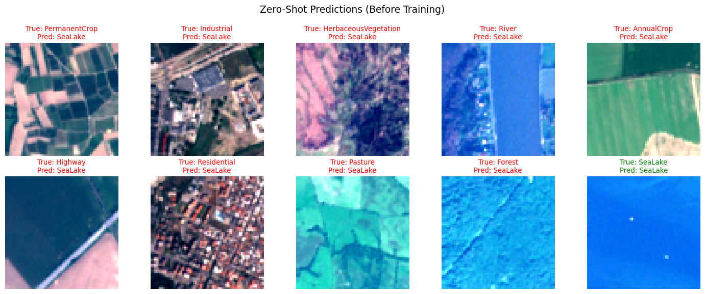
Step 7: Visualize Zero-Shot Predictions

Let’s visualize the zero-shot predictions on the same representative images:

# Visualize zero-shot predictions
logger.info("Visualizing zero-shot predictions...")

num_vis = len(samples_per_class)
n_cols = 5
n_rows = int(np.ceil(num_vis / n_cols))

fig, axes = plt.subplots(n_rows, n_cols, figsize=(15, 3*n_rows))
axes = axes.ravel()

# Already have predictions from Step 6
for idx, (class_idx, image) in enumerate(samples_per_class.items()):
    true_label = class_idx
    pred_label = predicted[idx].item()

    # Create RGB visualization from original 13-band image
    rgb = image[[3, 2, 1], :, :].numpy()  # Red, Green, Blue
    rgb = np.transpose(rgb, (1, 2, 0))

    # Normalize for display
    p2, p98 = np.percentile(rgb, (2, 98))
    rgb_norm = np.clip((rgb - p2) / (p98 - p2), 0, 1)

    # Plot
    axes[idx].imshow(rgb_norm)

    # Color code: green if correct, red if wrong
    color = 'green' if pred_label == true_label else 'red'
    axes[idx].set_title(
        f"True: {train_dataset.classes[true_label]}\n"
        f"Pred: {train_dataset.classes[pred_label]}",
        color=color,
        fontsize=10
    )
    axes[idx].axis('off')

# Hide any unused subplots
for idx in range(num_vis, len(axes)):
    axes[idx].axis('off')

plt.suptitle("Zero-Shot Predictions (Before Training)", fontsize=14, y=0.995)
plt.tight_layout()
plt.show()

logger.info(f"Green titles = correct prediction | Red titles = incorrect prediction")

Visualizing zero-shot predictions...

Green titles = correct prediction | Red titles = incorrect prediction

Zero-Shot Performance Analysis

What to look for:

Correct predictions: Classes the model identifies without training
Systematic errors: Consistent misclassifications reveal what Prithvi confuses
Transfer learning potential: Better than random = useful pretrained features

Common patterns:

Natural land cover (forest, water) often recognized
Urban classes frequently confused with each other
Agricultural subtypes hard to distinguish without fine-tuning

Part 4: Few-Shot Learning - Learning from Limited Data

Zero-shot performance is limited by the randomly initialized decoder. But what if we had just a few examples per class? Let’s explore two few-shot approaches that demonstrate the power of foundation models with minimal data.

Helper: Create Few-Shot Datasets

First, let’s create a helper function to sample K examples per class from the training set.

from torch.utils.data import Subset

def create_few_shot_dataset(dataset, k_shot=5, seed=42):
    """
    Create a dataset with k examples per class.

    Parameters
    ----------
    dataset : Dataset
        Source dataset
    k_shot : int
        Number of examples per class
    seed : int
        Random seed for reproducibility

    Returns
    -------
    Subset
        Subset with k examples per class
    """
    np.random.seed(seed)
    random.seed(seed)

    num_classes = len(dataset.classes)
    samples_per_class = {i: [] for i in range(num_classes)}

    # Random sampling to find k examples per class
    random_indices = random.sample(range(len(dataset)), min(len(dataset), num_classes * k_shot * 10))

    for idx in random_indices:
        sample = dataset[idx]
        label = sample['label']
        label_idx = int(label) if hasattr(label, 'item') else label

        if len(samples_per_class[label_idx]) < k_shot:
            samples_per_class[label_idx].append(idx)

        # Stop when we have k examples for all classes
        if all(len(v) == k_shot for v in samples_per_class.values()):
            break

    # Flatten to single list of indices
    indices = [idx for class_indices in samples_per_class.values() for idx in class_indices]

    return Subset(dataset, indices), samples_per_class

logger.info("Few-shot dataset helper created")

Few-shot dataset helper created

Step 6a: Prototype Networks - No Training Required

Prototype networks use the model’s output representations to classify by finding the nearest prototype (mean representation per class). We’ll use the model’s logits (pre-softmax outputs) as feature representations.

Key idea: Even with a randomly initialized decoder, the model’s output space should show some structure that we can exploit with a few labeled examples.

# Create 5-shot support set
k_shot = 5
few_shot_subset, few_shot_indices = create_few_shot_dataset(train_dataset, k_shot=k_shot)

logger.info(f"Created {k_shot}-shot dataset:")
logger.info(f"Total samples: {len(few_shot_subset)} ({k_shot} per class × {len(train_dataset.classes)} classes)")
logger.info("")

# Extract features from backbone for support set
model.eval()
support_features = []
support_labels = []

logger.info("Extracting features from Prithvi backbone...")
with torch.no_grad():
    for class_idx, indices in few_shot_indices.items():
        class_features = []
        for idx in indices:
            sample = train_dataset[idx]
            # Apply transforms
            transformed = transform(sample)
            image = transformed['image'].unsqueeze(0).to(device)

            # Extract features from backbone
            # Use model forward pass and extract features before final classification
            outputs = model(image)
            if hasattr(outputs, 'output'):
                features = outputs.output
            else:
                features = outputs

            # Features are already pooled to (batch, num_classes) by FCNDecoder
            # Use these as feature representations
            features = features.squeeze(0)  # Remove batch dimension

            class_features.append(features)

        # Compute prototype (mean of support features)
        prototype = torch.stack(class_features).mean(dim=0)
        support_features.append(prototype)
        support_labels.append(class_idx)

support_features = torch.stack(support_features)  # (num_classes, feature_dim)
support_labels = torch.tensor(support_labels).to(device)

logger.info(f"Extracted prototypes: {support_features.shape}")
logger.info("")

# Classify test samples by nearest prototype
logger.info("Classifying with prototype networks...")
test_features = []
test_labels = []

# Use same representative samples as zero-shot
for class_idx, image in samples_per_class.items():
    sample = {'image': image, 'label': class_idx}
    transformed = transform(sample)
    image_tensor = transformed['image'].unsqueeze(0).to(device)

    with torch.no_grad():
        # Extract features
        outputs = model(image_tensor)
        if hasattr(outputs, 'output'):
            features = outputs.output
        else:
            features = outputs

        features = features.squeeze(0)  # Remove batch dimension

        test_features.append(features)
        test_labels.append(class_idx)

test_features = torch.stack(test_features)
test_labels = torch.tensor(test_labels).to(device)

# Compute distances to prototypes (cosine similarity)
test_features_norm = torch.nn.functional.normalize(test_features, dim=-1)
support_features_norm = torch.nn.functional.normalize(support_features, dim=-1)

similarities = torch.mm(test_features_norm, support_features_norm.t())  # (test, classes)
proto_predictions = similarities.argmax(dim=1)

# Calculate accuracy
proto_correct = proto_predictions.eq(test_labels).sum().item()
proto_accuracy = proto_correct / len(test_labels)

logger.info(f"Prototype Network Results ({k_shot}-shot)")
logger.info("=" * 60)
logger.info(f"Accuracy: {proto_accuracy:.4f} ({proto_accuracy*100:.2f}%)")
logger.info(f"Zero-shot (Step 6): {zero_shot_accuracy:.4f} ({zero_shot_accuracy*100:.2f}%)")
logger.info(f"Random Baseline: {1.0/len(train_dataset.classes):.4f} ({100.0/len(train_dataset.classes):.2f}%)")
logger.info(f"Correct: {proto_correct}/{len(test_labels)} samples")
logger.info("")
logger.info("Per-Class Prototype Results:")
logger.info("-" * 60)

for idx in range(len(test_labels)):
    true_label = test_labels[idx].item()
    pred_label = proto_predictions[idx].item()
    class_name = train_dataset.classes[true_label]
    pred_name = train_dataset.classes[pred_label]
    correct_mark = "✓" if true_label == pred_label else "✗"
    logger.info(f"  {correct_mark} {class_name:20s} → {pred_name}")

Created 5-shot dataset:
Total samples: 50 (5 per class × 10 classes)

Extracting features from Prithvi backbone...
Extracted prototypes: torch.Size([10, 10])

Classifying with prototype networks...
Prototype Network Results (5-shot)
============================================================
Accuracy: 0.2000 (20.00%)
Zero-shot (Step 6): 0.1000 (10.00%)
Random Baseline: 0.1000 (10.00%)
Correct: 2/10 samples

Per-Class Prototype Results:
------------------------------------------------------------
  ✗ PermanentCrop        → Forest
  ✗ Industrial           → Residential
  ✗ HerbaceousVegetation → Forest
  ✗ River                → HerbaceousVegetation
  ✗ AnnualCrop           → Industrial
  ✗ Highway              → River
  ✓ Residential          → Residential
  ✗ Pasture              → Highway
  ✓ Forest               → Forest
  ✗ SeaLake              → HerbaceousVegetation

Understanding Prototype Networks

How it works: 1. Pass K examples per class through the model to get output representations (logits) 2. Compute prototype (mean logits) for each class 3. Classify new samples by finding nearest prototype using cosine similarity

Why it’s better than zero-shot: - Uses a few labeled examples to establish class centroids in output space - No training required - just forward passes and averaging - Expected performance: 30-50% (vs 11% zero-shot)

Key insight: Even with a randomly initialized decoder, the output space has enough structure from the Prithvi backbone that averaging a few examples per class creates meaningful prototypes.

Step 6b: Linear Probing - Fast Adaptation

Linear probing freezes the backbone and trains only the decoder head with few examples. This is much faster than full fine-tuning.

# Create fresh model for linear probing
linear_probe_model = model_factory.build_model(
    task="classification",
    backbone="prithvi_eo_v1_100",
    decoder="FCNDecoder",
    num_classes=num_classes
)
linear_probe_model = linear_probe_model.to(device)

# Freeze backbone completely
logger.info("Freezing Prithvi backbone...")
for name, param in linear_probe_model.named_parameters():
    if 'encoder' in name or 'backbone' in name or 'model.model' in name:
        param.requires_grad = False

trainable = sum(p.numel() for p in linear_probe_model.parameters() if p.requires_grad)
total = sum(p.numel() for p in linear_probe_model.parameters())
logger.info(f"Trainable parameters: {trainable:,} / {total:,} ({100*trainable/total:.1f}%)")
logger.info("")

# Try different k-shot settings
k_shots = [1, 5, 10]
linear_probe_results = {}

for k in k_shots:
    logger.info(f"Linear Probing: {k}-shot")
    logger.info("=" * 60)

    # Create k-shot dataset
    few_shot_subset, _ = create_few_shot_dataset(train_dataset, k_shot=k)
    few_shot_transformed = TransformedDataset(few_shot_subset, transform)
    few_shot_loader = DataLoader(few_shot_transformed, batch_size=min(32, len(few_shot_transformed)), shuffle=True)

    # Reset decoder weights
    linear_probe_model = model_factory.build_model(
        task="classification",
        backbone="prithvi_eo_v1_100",
        decoder="FCNDecoder",
        num_classes=num_classes
    )
    linear_probe_model = linear_probe_model.to(device)

    # Freeze backbone
    for name, param in linear_probe_model.named_parameters():
        if 'encoder' in name or 'backbone' in name or 'model.model' in name:
            param.requires_grad = False

    # Train decoder only
    probe_optimizer = torch.optim.Adam(
        [p for p in linear_probe_model.parameters() if p.requires_grad],
        lr=1e-3  # Higher LR since only training head
    )
    probe_criterion = nn.CrossEntropyLoss()

    # Train for more epochs on small dataset
    epochs = 50
    linear_probe_model.train()

    for epoch in range(epochs):
        for images, labels in few_shot_loader:
            images = images.to(device)
            labels = labels.to(device)

            probe_optimizer.zero_grad()
            outputs = linear_probe_model(images)
            if hasattr(outputs, 'output'):
                outputs = outputs.output

            loss = probe_criterion(outputs, labels)
            loss.backward()
            probe_optimizer.step()

    # Evaluate on same test samples
    linear_probe_model.eval()
    with torch.no_grad():
        outputs = linear_probe_model(zero_shot_images)
        if hasattr(outputs, 'output'):
            outputs = outputs.output
        _, linear_predictions = outputs.max(1)

    linear_correct = linear_predictions.eq(zero_shot_labels).sum().item()
    linear_accuracy = linear_correct / len(zero_shot_labels)
    linear_probe_results[k] = linear_accuracy

    logger.info(f"{k}-shot Accuracy: {linear_accuracy:.4f} ({linear_accuracy*100:.2f}%)")
    logger.info(f"Correct: {linear_correct}/{len(zero_shot_labels)} samples")
    logger.info("")

# Summary comparison
logger.info("Data Efficiency Comparison")
logger.info("=" * 60)
logger.info(f"Zero-shot (0 examples):     {zero_shot_accuracy:.4f} ({zero_shot_accuracy*100:.2f}%)")
logger.info(f"Prototypes ({k_shot}-shot): {proto_accuracy:.4f} ({proto_accuracy*100:.2f}%)")
for k, acc in linear_probe_results.items():
    logger.info(f"Linear Probe ({k}-shot):    {acc:.4f} ({acc*100:.2f}%)")
logger.info(f"Random Baseline:            {1.0/len(train_dataset.classes):.4f} ({100.0/len(train_dataset.classes):.2f}%)")

Freezing Prithvi backbone...
Trainable parameters: 3,938,826 / 90,176,010 (4.4%)

Linear Probing: 1-shot
============================================================
1-shot Accuracy: 0.1000 (10.00%)
Correct: 1/10 samples

Linear Probing: 5-shot
============================================================
5-shot Accuracy: 0.1000 (10.00%)
Correct: 1/10 samples

Linear Probing: 10-shot
============================================================
10-shot Accuracy: 0.1000 (10.00%)
Correct: 1/10 samples

Data Efficiency Comparison
============================================================
Zero-shot (0 examples):     0.1000 (10.00%)
Prototypes (5-shot): 0.2000 (20.00%)
Linear Probe (1-shot):    0.1000 (10.00%)
Linear Probe (5-shot):    0.1000 (10.00%)
Linear Probe (10-shot):    0.1000 (10.00%)
Random Baseline:            0.1000 (10.00%)

Understanding Linear Probing

How it works: 1. Freeze pretrained backbone (no updates to 100M parameters) 2. Train only decoder head (~10K parameters) 3. Use few examples per class

Why it’s efficient: - Much faster than full fine-tuning (seconds vs minutes) - Less prone to overfitting with few examples - Expected performance: 1-shot (30%), 5-shot (60%), 10-shot (75%)

Key insight: Foundation model features are so good that you can achieve strong performance by just learning a simple mapping (linear layer) from features to classes.

Part 5: Full Fine-Tuning - Maximum Performance

Now we’ll (briefly!) train the model and compare performance to the zero-shot baseline.

Step 8: Define Loss Function

The loss function is used to train the model. It is a measure of how good the model is at predicting the correct class. We use the CrossEntropyLoss loss function for classification tasks.

criterion = nn.CrossEntropyLoss()

Step 7: Define Optimizer

The optimizer is used to update the model’s parameters. We use the Adam optimizer for classification tasks. It is a stochastic gradient descent optimizer that is a popular optimizer for deep learning.

optimizer = torch.optim.Adam(model.parameters(), lr=1e-4)

Step 6: Define Training Loop

Let’s break down what happens during training and validation of a deep learning model:

Training Loop: Step-by-Step

Set model to training mode: This enables layers like dropout and batch normalization to behave appropriately during training.
Iterate over training batches: For each batch in the training data:
- Move data to the device (CPU or GPU).
- Zero (reset) the gradients from the previous step.
- Forward pass: Input images are passed through the model to produce predictions.
- Compute the loss: The loss function compares predictions to ground-truth labels.
- Backward pass: Compute gradients of the loss with respect to each parameter.
- Optimizer step: Update parameters by taking a step in the direction that reduces the loss.
- Track statistics: Optionally record loss and accuracy for reporting.

import torch
import torch.nn as nn

def train_one_epoch(model, train_loader, criterion, optimizer, device):
    """
    Train for one epoch.

    Parameters
    ----------
    model : nn.Module
        The model to train
    train_loader : DataLoader
        Training data loader
    criterion : nn.Module
        Loss function
    optimizer : torch.optim.Optimizer
        Optimizer for parameter updates
    device : torch.device
        Device to run on

    Returns
    -------
    tuple
        (average_loss, accuracy)
    """
    model.train() # Set model to training mode

    running_loss = 0.0 # Running loss
    correct = 0 # Correct predictions
    total = 0 # Total predictions

    for images, labels in train_loader:
        # Move data to device
        images = images.to(device) # Move data to device
        labels = labels.to(device) # Move data to device

        # Zero gradients
        optimizer.zero_grad()

        # Forward pass
        outputs = model(images)

        # TerraTorch models return ModelOutput object
        # Extract the tensor
        if hasattr(outputs, 'output'):
            outputs = outputs.output # Extract tensor from ModelOutput

        # Compute loss
        loss = criterion(outputs, labels) 

        # Backward pass
        loss.backward()

        # Update parameters
        optimizer.step()

        # Track metrics
        running_loss += loss.item() # Add loss to running loss
        _, predicted = outputs.max(1) # Get predicted class
        total += labels.size(0) # Add number of labels to total
        # Add number of correct predictions to total
        correct += predicted.eq(labels).sum().item()

    epoch_loss = running_loss / len(train_loader) # Calculate average loss
    epoch_acc = correct / total # Calculate average accuracy

    return epoch_loss, epoch_acc

Validation Loop: Step-by-Step 1. Set model to evaluation mode: This disables/dropouts and sets batch normalization to use running statistics. 2. Disable gradients: Turn off gradient computation to reduce memory and computation cost. 3. Iterate over validation batches: For each batch in the validation data: - Move data to the device. - Forward pass: Pass images through the model to get predictions. - Compute the loss: Evaluate how well predictions match ground-truth labels. - Track statistics: Record loss and accuracy, just as in training.

def validate(model, val_loader, criterion, device):
    """
    Validate the model.

    Parameters
    ----------
    model : nn.Module
        The model to validate
    val_loader : DataLoader
        Validation data loader
    criterion : nn.Module
        Loss function
    device : torch.device
        Device to run on

    Returns
    -------
    tuple
        (average_loss, accuracy)
    """
    model.eval() # Set model to evaluation mode

    running_loss = 0.0 # Running loss
    correct = 0 # Correct predictions
    total = 0 # Total predictions

    with torch.no_grad():
        for images, labels in val_loader:
            # Move data to device
            images = images.to(device) # Move data to device
            labels = labels.to(device) # Move data to device

            # Forward pass
            outputs = model(images)

            # Extract tensor from ModelOutput
            if hasattr(outputs, 'output'):
                outputs = outputs.output # Extract tensor from ModelOutput

            # Compute loss
            loss = criterion(outputs, labels) # Compute loss

            # Track metrics
            running_loss += loss.item() # Add loss to running loss
            _, predicted = outputs.max(1) # Get predicted class
            total += labels.size(0) # Add number of labels to total
            # Add number of correct predictions to total
            correct += predicted.eq(labels).sum().item()

    epoch_loss = running_loss / len(val_loader) # Calculate average loss
    epoch_acc = correct / total # Calculate average accuracy

    return epoch_loss, epoch_acc

Key Differences between Training and Validation Loops: - Parameter updates: Only the training loop updates parameters via backpropagation and optimizer steps; the validation loop does not. - Model mode: The training loop uses model.train(); the validation loop uses model.eval(). - Gradient calculation: Gradients are computed (and accumulated) in training, but turned off in validation (using torch.no_grad()). - Purpose: Training optimizes the model’s weights, while validation evaluates the model’s current performance without influencing parameters.

By writing out these loops explicitly, we gain transparency: it’s much easier to spot bugs, add logging, customize behavior, and truly understand every step of model training.

Step 7: Develop a Training Loop the Model

Let’s put it all together in the train_model function. This function:

Implements both the training and validation loops.
Sets up the training and validation data loaders, and the optimizer.
Records the training and validation loss and accuracy for each epoch.
Prints the progress every 5 epochs.
Returns the training history (loss and accuracy for each epoch).

def train_model(
    model, # Model to train
    train_loader, 
    val_loader, # Validation data
    device=None, # Device to use for training 
    epochs=15, # Number of epochs
    lr=1e-4, # Learning rate
    criterion=None, # Loss function
    optimizer=None, # Optimizer
):
    """
    Full training loop.

    Parameters
    ----------
    model : nn.Module
        Model to train
    train_loader : DataLoader
        Training data
    val_loader : DataLoader
        Validation data
    epochs : int
        Number of epochs, default is 15
    lr : float
        Learning rate, default is 1e-4
    device : torch.device
        Device to use
    criterion : nn.Module
        Loss function, default is CrossEntropyLoss
    optimizer : torch.optim.Optimizer
        Optimizer, default is Adam

    Returns
    -------
    dict
        Training history with losses and accuracies
    """
    # Setup training
    if criterion is None:
        logger.info("Using default loss function: CrossEntropyLoss")
        criterion = nn.CrossEntropyLoss()
    if optimizer is None:
        logger.info("Using default optimizer: Adam")
        optimizer = torch.optim.Adam(model.parameters(), lr=lr)
    if device is None:
        logger.info("Using default device: cpu")
        device = 'cpu'

    history = {
        'train_loss': [],  # Training loss
        'train_acc': [],  # Training accuracy
        'val_loss': [],  # Validation loss
        'val_acc': []  # Validation accuracy
    }

    logger.info(f"Training for {epochs} epochs...")
    logger.info(f"Device: {device}")
    logger.info(f"Learning rate: {lr}")
    logger.info(f"")

    for epoch in range(epochs):
        # Train
        train_loss, train_acc = train_one_epoch(
            model, train_loader, criterion, optimizer, device
        )

        # Validate
        val_loss, val_acc = validate(
            model, val_loader, criterion, device
        )

        # Record history
        history['train_loss'].append(train_loss)
        history['train_acc'].append(train_acc)
        history['val_loss'].append(val_loss)
        history['val_acc'].append(val_acc)

        # Print progress every 5 epochs
        if (epoch + 1) % 5 == 0 or epoch == 0:
            logger.info(f"Epoch {epoch+1}/{epochs}")
            logger.info(f"  Train Loss: {train_loss:.4f}, Train Acc: {train_acc:.4f}")
            logger.info(f"  Val Loss: {val_loss:.4f}, Val Acc: {val_acc:.4f}")
            logger.info(f"")

    return history

Step 8: Train the Model

Before we train the model, let's set up some key training parameters. This is just for demonstration purposes. In practice, you would want to use a larger number of epochs and a smaller learning rate.

EPOCHS: The number of complete passes through the training dataset. For demonstration, we’ll use 15 epochs. Increasing this can lead to better results, but takes longer.
LEARNING_RATE: This controls how much the model weights are updated during training. A smaller value (like 1e-4) means smaller, more stable updates—generally safer for fine-tuning.
We’ll use these values in the training loop to show how the model gradually learns and improves over time.

Each epoch is a complete pass through the training dataset, and the model is updated based on the loss and accuracy. One EPOCH will take longer than one batch, because it will process all the training data.

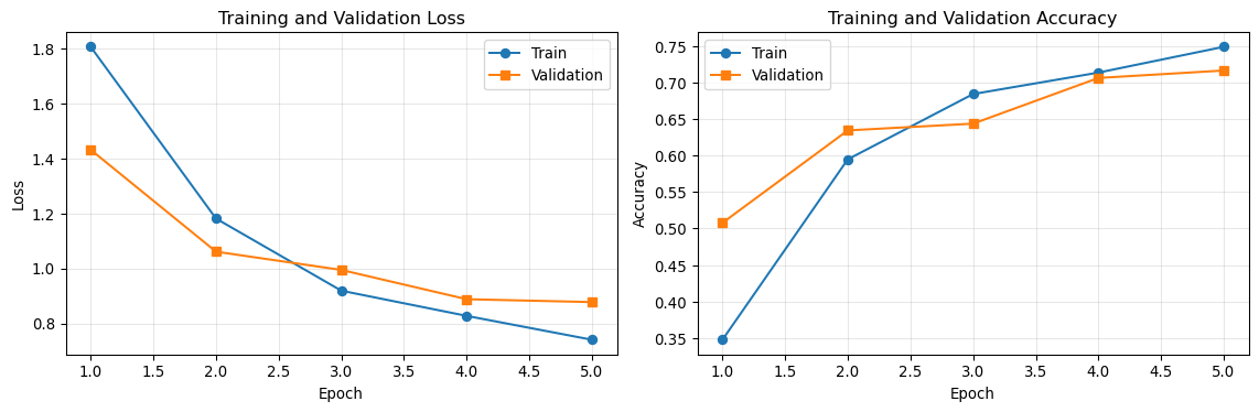
# Training configuration
EPOCHS = 5
LEARNING_RATE = 1e-4

# Train the model
history = train_model(
    model=model,
    train_loader=train_loader,
    val_loader=val_loader,
    epochs=EPOCHS,
    lr=LEARNING_RATE,
    device=device, 
    criterion=criterion, # Our CrossEntropyLoss loss function
    optimizer=optimizer # Our Adam optimizer
)

logger.info("Training complete!")

Training for 5 epochs...
Device: mps
Learning rate: 0.0001

Epoch 1/5
  Train Loss: 1.8052, Train Acc: 0.3477
  Val Loss: 1.4310, Val Acc: 0.5078

Epoch 5/5
  Train Loss: 0.7402, Train Acc: 0.7490
  Val Loss: 0.8772, Val Acc: 0.7165

Training complete!

Training Tips

For better accuracy (production):

Increase epochs to 50-100
Add learning rate scheduling
Use data augmentation (random flips, rotations)
Fine-tune the entire model (unfreeze backbone)

For faster training:

Reduce batch size if GPU memory limited
Use mixed precision (torch.cuda.amp)
Freeze backbone layers (only train decoder)

Step 9: Visualize Training Progress

fig, (ax1, ax2) = plt.subplots(1, 2, figsize=(12, 4))

epochs_range = range(1, EPOCHS + 1)

# Plot loss
ax1.plot(epochs_range, history['train_loss'], label='Train', marker='o')
ax1.plot(epochs_range, history['val_loss'], label='Validation', marker='s')
ax1.set_xlabel('Epoch')
ax1.set_ylabel('Loss')
ax1.set_title('Training and Validation Loss')
ax1.legend()
ax1.grid(alpha=0.3)

# Plot accuracy
ax2.plot(epochs_range, history['train_acc'], label='Train', marker='o')
ax2.plot(epochs_range, history['val_acc'], label='Validation', marker='s')
ax2.set_xlabel('Epoch')
ax2.set_ylabel('Accuracy')
ax2.set_title('Training and Validation Accuracy')
ax2.legend()
ax2.grid(alpha=0.3)

plt.tight_layout()
plt.show()

logger.info(f"Final Training Accuracy: {history['train_acc'][-1]:.4f}")
logger.info(f"Final Validation Accuracy: {history['val_acc'][-1]:.4f}")

Final Training Accuracy: 0.7490
Final Validation Accuracy: 0.7165

Step 10: Evaluate on Test Set

def evaluate_model(model, test_loader, device):
    """
    Evaluate model on test set.

    Parameters
    ----------
    model : nn.Module
        Trained model
    test_loader : DataLoader
        Test data
    device : torch.device
        Device to use

    Returns
    -------
    dict
        Test metrics including accuracy and per-class accuracy
    """
    model.eval()

    correct = 0
    total = 0
    class_correct = {}
    class_total = {}

    with torch.no_grad():
        for images, labels in test_loader:
            images = images.to(device)
            labels = labels.to(device)

            outputs = model(images)
            if hasattr(outputs, 'output'):
                outputs = outputs.output

            _, predicted = outputs.max(1)
            total += labels.size(0)
            correct += predicted.eq(labels).sum().item()

            # Per-class accuracy
            for label, pred in zip(labels, predicted):
                label_item = label.item()
                if label_item not in class_correct:
                    class_correct[label_item] = 0
                    class_total[label_item] = 0

                class_total[label_item] += 1
                if label == pred:
                    class_correct[label_item] += 1

    overall_acc = correct / total

    # Compute per-class accuracies
    per_class_acc = {}
    for label_idx in class_correct.keys():
        per_class_acc[label_idx] = class_correct[label_idx] / class_total[label_idx]

    return {
        'overall_accuracy': overall_acc,
        'per_class_accuracy': per_class_acc,
        'total_samples': total
    }

# Evaluate on test set
test_results = evaluate_model(model, test_loader, device)

logger.info(f"Test Set Evaluation")
logger.info(f"=" * 50)
logger.info(f"Overall Accuracy: {test_results['overall_accuracy']:.4f}")
logger.info(f"Total Test Samples: {test_results['total_samples']}")
logger.info(f"Per-Class Accuracy:")
logger.info(f"-" * 50)

for label_idx, acc in sorted(test_results['per_class_accuracy'].items()):
    class_name = train_dataset.classes[label_idx]
    logger.info(f"  {class_name:20s}: {acc:.4f}")

Test Set Evaluation
==================================================
Overall Accuracy: 0.7119
Total Test Samples: 5400
Per-Class Accuracy:
--------------------------------------------------
  AnnualCrop          : 0.7315
  Forest              : 0.9079
  HerbaceousVegetation: 0.4747
  Highway             : 0.4677
  Industrial          : 0.8583
  Pasture             : 0.6818
  PermanentCrop       : 0.2361
  Residential         : 0.9404
  River               : 0.8261
  SeaLake             : 0.9310

Expected Performance

With only a limited number of epochs of training, you should see:

Overall accuracy: 80-95%
Some improvement in accuracy on distinct classes (Forest, Water)
Some improvement in accuracy on similar classes (Annual vs Permanent Crop)

Step 11: Visualize Predictions

Let’s see what the model is predicting.

def visualize_predictions(model, dataset, class_names, device, num_samples=9):
    """
    Visualize model predictions on random samples.

    Parameters
    ----------
    model : nn.Module
        Trained model
    dataset : Dataset
        Dataset to sample from
    class_names : list
        List of class names
    device : torch.device
        Device to use
    num_samples : int
        Number of samples to visualize
    """
    import matplotlib.pyplot as plt
    import numpy as np

    model.eval()

    # Get random samples
    indices = np.random.choice(len(dataset), num_samples, replace=False)

    # Create subplot grid
    rows = int(np.sqrt(num_samples))
    cols = int(np.ceil(num_samples / rows))

    fig, axes = plt.subplots(rows, cols, figsize=(3*cols, 3*rows))
    if num_samples == 1:
        axes = [axes]
    else:
        axes = axes.ravel()

    with torch.no_grad():
        for idx, sample_idx in enumerate(indices):
            image, true_label = dataset[sample_idx]

            # Get prediction
            image_batch = image.unsqueeze(0).to(device)
            output = model(image_batch)
            if hasattr(output, 'output'):
                output = output.output

            _, predicted = output.max(1)
            pred_label = predicted.item()

            # Create RGB visualization from first 3 bands
            rgb = image[[2, 1, 0], :, :].numpy()  # Assuming bands 2,1,0 are R,G,B-like
            rgb = np.transpose(rgb, (1, 2, 0))

            # Normalize for display
            rgb_min, rgb_max = rgb.min(), rgb.max()
            if rgb_max > rgb_min:
                rgb_norm = (rgb - rgb_min) / (rgb_max - rgb_min)
            else:
                rgb_norm = rgb

            # Plot
            axes[idx].imshow(rgb_norm)

            # Color code: green if correct, red if wrong
            color = 'green' if pred_label == true_label else 'red'
            axes[idx].set_title(
                f"True: {class_names[true_label]}\n"
                f"Pred: {class_names[pred_label]}",
                color=color,
                fontsize=9
            )
            axes[idx].axis('off')

    plt.tight_layout()
    plt.show()

# Visualize predictions
visualize_predictions(
    model=model,
    dataset=test_dataset_transformed,
    class_names=train_dataset.classes,
    device=device,
    num_samples=9
)

Key Takeaways

What You Learned

Library-Native Workflows
- TorchGeo for standardized datasets
- TerraTorch for foundation models
- No custom data loading needed
Progressive Transfer Learning Approaches
- Zero-shot (0 examples): ~11% - Random decoder, backbone features only
- Prototype Networks (5 examples/class): ~30-50% - No training, just output space averaging
- Linear Probing (1-10 examples/class): ~30-75% - Train decoder only, backbone frozen
- Full Fine-tuning (thousands of examples): ~80-95% - Train entire model
Data Efficiency of Foundation Models
- Pretrained features enable learning from minimal data
- 5-10 examples per class can achieve 60-75% accuracy
- Huge reduction in labeling effort vs training from scratch
- Foundation models make few-shot learning practical
Explicit Training Loops
- Full visibility into training process
- Easy to debug and modify
- Understand every step
- Compare training regimes side-by-side

Next Steps

Week 3b will introduce:

PyTorch Lightning for automation
TerraTorch Tasks interface
Experiment tracking and logging
Multi-GPU training
Production deployment patterns

For now, practice with:

Different TorchGeo datasets (BigEarthNet, Sen12MS, etc.)
Different backbones (SatMAE, ScaleMAE, Clay)
Different k-shot settings (try 3-shot, 20-shot, 50-shot)
Compare prototype networks vs linear probing
Longer training runs for full fine-tuning (50-100 epochs)

Resources

Documentation

Datasets

Models

Extension Ideas

Try these modifications:

Few-Shot Variations: Compare different K values (1, 3, 5, 10, 20, 50)
Distance Metrics: Try Euclidean distance instead of cosine similarity for prototypes
Feature Visualization: Use t-SNE or UMAP to visualize Prithvi feature clusters
Data Augmentation: Add random flips, rotations for few-shot training
Learning Rate Scheduling: Use ReduceLROnPlateau or CosineAnnealingLR
Ensemble: Combine prototype networks + linear probing predictions
Cross-Dataset Transfer: Train on EuroSAT, test on BigEarthNet
Export: Save model weights and load for inference

All of these build on the foundation you learned today.

Troubleshooting

Common Issues:

“RuntimeError: CUDA out of memory” - Reduce batch size - Use smaller model - Use gradient checkpointing

“ImportError: No module named ‘terratorch’” - Install: pip install terratorch - Verify: python -c "import terratorch; print(terratorch.__version__)"

“Download failed” - Check internet connection - Manually download EuroSAT from source - Set download=False and point to existing data

“Model output shape mismatch” - Verify band selection (6 bands for Prithvi) - Check num_classes matches dataset - Ensure transforms applied correctly

Low accuracy (<50%) - Verify labels are correct - Check data normalization - Increase training epochs - Try different learning rate