Week 3: Machine Learning on Remote Sensing

Introduction

This week we’ll train convolutional neural networks on real satellite imagery for land cover classification. You’ll experience the complete machine learning workflow: from patch extraction to model evaluation.

Learning Goals

By the end of this session, you will: - Extract training patches from preprocessed satellite data - Create labeled datasets for supervised learning - Build and train multiple CNN architectures - Compare model performance and interpret results - Understand the end-to-end ML workflow for remote sensing

Session Overview

Today’s hands-on machine learning pipeline:

Step	Activity	Tools	Output
1	Patch extraction from data cubes	numpy, sklearn	Training patches
2	Dataset creation and labeling	PyTorch, TorchGeo	Labeled datasets
3	CNN architecture comparison	PyTorch, torchvision	Multiple models
4	Training and validation	PyTorch, matplotlib	Trained models
5	Performance evaluation	sklearn, seaborn	Model comparison

---

Step 1: Patch Extraction from Preprocessed Data

Let’s start by extracting training patches from the data cubes we created in Week 2.

Load Preprocessed Data

import warnings
warnings.filterwarnings('ignore')

# Core libraries
import numpy as np
import pandas as pd
import xarray as xr
import matplotlib.pyplot as plt
import seaborn as sns
from pathlib import Path
from sklearn.model_selection import train_test_split
from sklearn.metrics import classification_report, confusion_matrix, accuracy_score
from sklearn.preprocessing import LabelEncoder

# Deep learning
import torch
import torch.nn as nn
import torch.optim as optim
import torch.nn.functional as F
from torch.utils.data import Dataset, DataLoader, TensorDataset
import torchvision.transforms as transforms
from torchvision.models import resnet18, resnet34

# Geospatial
import rasterio
import rioxarray

print("🔧 Libraries loaded for machine learning on remote sensing")

# Check if we have preprocessed data from Week 2
data_dir = Path("week2_preprocessed")
if data_dir.exists():
    cube_files = list(data_dir.glob("*cube*.nc"))
    if cube_files:
        cube_path = cube_files[0]
        print(f"📦 Loading data cube: {cube_path.name}")
        datacube = xr.open_dataset(cube_path)
        print(f"✅ Data cube loaded with shape: {datacube.dims}")
    else:
        print("⚠️ No data cube found, creating synthetic data for demonstration")
        datacube = None
else:
    print("⚠️ No preprocessed data directory found, creating synthetic data")
    datacube = None

🔧 Libraries loaded for machine learning on remote sensing
⚠️ No data cube found, creating synthetic data for demonstration

Create Training Data from Real or Synthetic Imagery

def create_training_patches(datacube=None, patch_size=64, n_patches_per_class=200):
    """
    Extract training patches for land cover classification.

    Args:
        datacube: xarray Dataset with satellite data
        patch_size: Size of patches to extract
        n_patches_per_class: Number of patches per class

    Returns:
        patches: Array of patches (N, C, H, W)
        labels: Array of class labels
        class_names: List of class names
    """

    # Define land cover classes
    class_names = [
        'Water',
        'Urban/Built-up',
        'Bare Soil/Rock',
        'Grassland/Pasture',
        'Cropland',
        'Forest'
    ]

    n_classes = len(class_names)
    n_bands = 4  # RGB + NIR

    if datacube is not None:
        # Use real data from datacube
        print("🌍 Using real satellite data for training patches")

        # Take median across time dimension if available
        if 'time' in datacube.dims:
            data = datacube.median(dim='time', skipna=True)
        else:
            data = datacube

        # Get RGB + NIR bands
        bands = ['red', 'green', 'blue', 'nir']

        # Extract patches from real data
        patches = []
        labels = []

        height, width = data['red'].shape

        # Simple land cover classification based on NDVI and other indices
        ndvi = (data['nir'] - data['red']) / (data['nir'] + data['red'] + 1e-8)
        red_intensity = data['red'] / (data['red'] + data['green'] + data['blue'] + 1e-8)

        for class_idx, class_name in enumerate(class_names):
            patches_extracted = 0
            attempts = 0
            max_attempts = n_patches_per_class * 10

            while patches_extracted < n_patches_per_class and attempts < max_attempts:
                # Random location
                y = np.random.randint(0, height - patch_size)
                x = np.random.randint(0, width - patch_size)

                # Extract patch location statistics
                patch_ndvi = ndvi.isel(y=slice(y, y+patch_size), x=slice(x, x+patch_size))
                patch_red = red_intensity.isel(y=slice(y, y+patch_size), x=slice(x, x+patch_size))

                # Skip if too many NaN values
                if np.isnan(patch_ndvi.values).sum() > patch_size**2 * 0.2:
                    attempts += 1
                    continue

                # Simple heuristic classification
                mean_ndvi = np.nanmean(patch_ndvi.values)
                mean_red = np.nanmean(patch_red.values)

                # Class assignment heuristics
                assigned_class = None
                if mean_ndvi < -0.1:  # Water
                    assigned_class = 0
                elif mean_red > 0.4 and mean_ndvi < 0.2:  # Urban/Built-up
                    assigned_class = 1
                elif mean_ndvi < 0.1:  # Bare Soil/Rock
                    assigned_class = 2
                elif 0.1 <= mean_ndvi < 0.3:  # Grassland/Pasture
                    assigned_class = 3
                elif 0.3 <= mean_ndvi < 0.6:  # Cropland
                    assigned_class = 4
                elif mean_ndvi >= 0.6:  # Forest
                    assigned_class = 5

                # Accept patch if it matches current class
                if assigned_class == class_idx:
                    # Extract patch for all bands
                    patch = np.stack([
                        data[band].isel(y=slice(y, y+patch_size), x=slice(x, x+patch_size)).values
                        for band in bands
                    ])

                    # Skip if patch has NaN values
                    if not np.isnan(patch).any():
                        patches.append(patch)
                        labels.append(class_idx)
                        patches_extracted += 1

                attempts += 1

            print(f"   {class_name}: {patches_extracted} patches extracted")

        patches = np.array(patches)
        labels = np.array(labels)

    else:
        # Create synthetic data for demonstration
        print("🎨 Creating synthetic satellite data for training patches")

        total_patches = n_patches_per_class * n_classes
        patches = np.zeros((total_patches, n_bands, patch_size, patch_size))
        labels = np.zeros(total_patches, dtype=int)

        for class_idx, class_name in enumerate(class_names):
            start_idx = class_idx * n_patches_per_class
            end_idx = start_idx + n_patches_per_class

            for i in range(start_idx, end_idx):
                # Create synthetic spectral signatures for each class
                if class_idx == 0:  # Water
                    # Low reflectance, especially in NIR
                    patches[i, 0] = np.random.normal(0.02, 0.01, (patch_size, patch_size))  # Red
                    patches[i, 1] = np.random.normal(0.03, 0.01, (patch_size, patch_size))  # Green
                    patches[i, 2] = np.random.normal(0.05, 0.015, (patch_size, patch_size)) # Blue
                    patches[i, 3] = np.random.normal(0.01, 0.005, (patch_size, patch_size)) # NIR
                elif class_idx == 1:  # Urban
                    # Moderate reflectance across all bands
                    patches[i, 0] = np.random.normal(0.15, 0.05, (patch_size, patch_size))
                    patches[i, 1] = np.random.normal(0.12, 0.04, (patch_size, patch_size))
                    patches[i, 2] = np.random.normal(0.08, 0.03, (patch_size, patch_size))
                    patches[i, 3] = np.random.normal(0.18, 0.06, (patch_size, patch_size))
                elif class_idx == 2:  # Bare soil
                    # Higher red, lower NIR
                    patches[i, 0] = np.random.normal(0.25, 0.08, (patch_size, patch_size))
                    patches[i, 1] = np.random.normal(0.20, 0.06, (patch_size, patch_size))
                    patches[i, 2] = np.random.normal(0.15, 0.05, (patch_size, patch_size))
                    patches[i, 3] = np.random.normal(0.22, 0.07, (patch_size, patch_size))
                elif class_idx == 3:  # Grassland
                    # Moderate vegetation signature
                    patches[i, 0] = np.random.normal(0.10, 0.03, (patch_size, patch_size))
                    patches[i, 1] = np.random.normal(0.15, 0.04, (patch_size, patch_size))
                    patches[i, 2] = np.random.normal(0.08, 0.02, (patch_size, patch_size))
                    patches[i, 3] = np.random.normal(0.30, 0.08, (patch_size, patch_size))
                elif class_idx == 4:  # Cropland
                    # Strong vegetation signature
                    patches[i, 0] = np.random.normal(0.08, 0.02, (patch_size, patch_size))
                    patches[i, 1] = np.random.normal(0.12, 0.03, (patch_size, patch_size))
                    patches[i, 2] = np.random.normal(0.06, 0.02, (patch_size, patch_size))
                    patches[i, 3] = np.random.normal(0.45, 0.10, (patch_size, patch_size))
                elif class_idx == 5:  # Forest
                    # Very strong vegetation signature
                    patches[i, 0] = np.random.normal(0.06, 0.015, (patch_size, patch_size))
                    patches[i, 1] = np.random.normal(0.10, 0.025, (patch_size, patch_size))
                    patches[i, 2] = np.random.normal(0.04, 0.01, (patch_size, patch_size))
                    patches[i, 3] = np.random.normal(0.55, 0.12, (patch_size, patch_size))

                # Add some spatial structure (texture)
                for band in range(n_bands):
                    # Add some texture/patterns
                    texture = np.random.normal(0, 0.01, (patch_size, patch_size))
                    patches[i, band] += texture

                labels[i] = class_idx

            print(f"   {class_name}: {n_patches_per_class} patches created")

    # Ensure positive values and reasonable range
    patches = np.clip(patches, 0, 1)

    print(f"\n📊 Dataset created:")
    print(f"   Total patches: {len(patches)}")
    print(f"   Patch shape: {patches.shape[1:]}")
    print(f"   Classes: {n_classes}")

    return patches, labels, class_names

# Create training data
patches, labels, class_names = create_training_patches(datacube, patch_size=64, n_patches_per_class=150)

🎨 Creating synthetic satellite data for training patches
   Water: 150 patches created
   Urban/Built-up: 150 patches created
   Bare Soil/Rock: 150 patches created
   Grassland/Pasture: 150 patches created
   Cropland: 150 patches created
   Forest: 150 patches created

📊 Dataset created:
   Total patches: 900
   Patch shape: (4, 64, 64)
   Classes: 6

Visualize Training Data

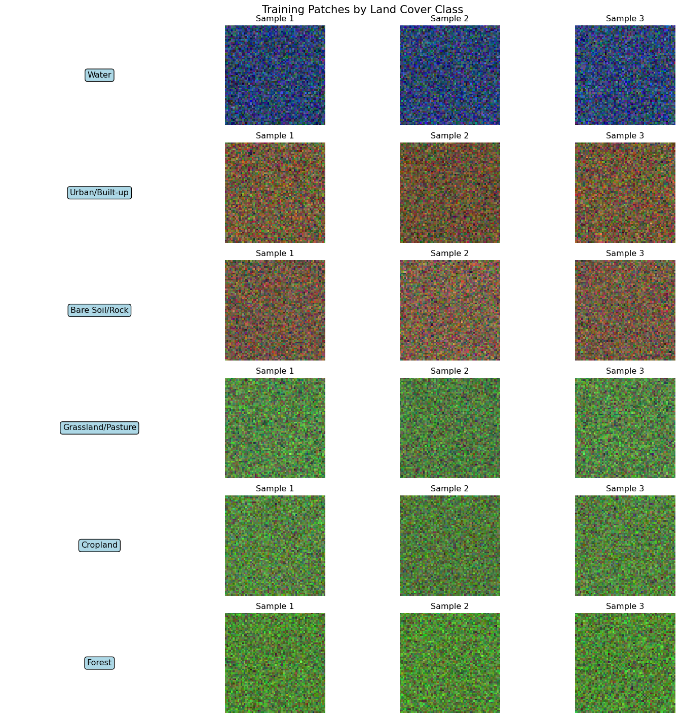
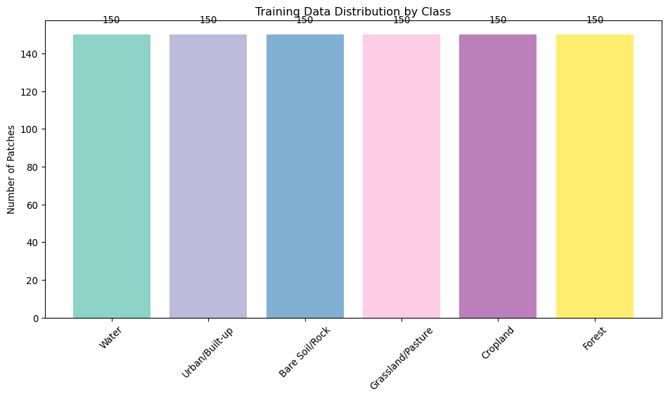
def visualize_training_samples(patches, labels, class_names, n_samples=3):
    """Visualize sample patches for each class."""

    n_classes = len(class_names)
    fig, axes = plt.subplots(n_classes, n_samples + 1, figsize=(15, 2.5 * n_classes))

    for class_idx, class_name in enumerate(class_names):
        # Find samples for this class
        class_mask = labels == class_idx
        class_patches = patches[class_mask]

        if len(class_patches) == 0:
            continue

        # Class label
        axes[class_idx, 0].text(0.5, 0.5, class_name,
                               transform=axes[class_idx, 0].transAxes,
                               fontsize=12, ha='center', va='center',
                               bbox=dict(boxstyle="round,pad=0.3", facecolor="lightblue"))
        axes[class_idx, 0].axis('off')

        # Sample patches
        for sample_idx in range(n_samples):
            if sample_idx < len(class_patches):
                patch = class_patches[sample_idx]

                # Create RGB composite (assuming bands 0,1,2 are R,G,B)
                rgb = patch[:3].transpose(1, 2, 0)

                # Normalize for display
                rgb_norm = np.clip((rgb - rgb.min()) / (rgb.max() - rgb.min() + 1e-8), 0, 1)

                axes[class_idx, sample_idx + 1].imshow(rgb_norm)
                axes[class_idx, sample_idx + 1].axis('off')
                axes[class_idx, sample_idx + 1].set_title(f'Sample {sample_idx + 1}')
            else:
                axes[class_idx, sample_idx + 1].axis('off')

    plt.suptitle('Training Patches by Land Cover Class', fontsize=16)
    plt.tight_layout()
    plt.show()

# Visualize sample patches
visualize_training_samples(patches, labels, class_names)

# Show class distribution
plt.figure(figsize=(10, 6))
unique_labels, counts = np.unique(labels, return_counts=True)
bars = plt.bar([class_names[i] for i in unique_labels], counts,
               color=plt.cm.Set3(np.linspace(0, 1, len(unique_labels))))
plt.title('Training Data Distribution by Class')
plt.ylabel('Number of Patches')
plt.xticks(rotation=45)

# Add count labels on bars
for bar, count in zip(bars, counts):
    plt.text(bar.get_x() + bar.get_width()/2, bar.get_height() + 5,
             str(count), ha='center', va='bottom')

plt.tight_layout()
plt.show()

print(f"📈 Class distribution visualization complete")

📈 Class distribution visualization complete

---

Step 2: Dataset Creation and Preparation

Now let’s prepare our data for PyTorch training with proper train/validation splits.

Create PyTorch Dataset

class SatelliteDataset(Dataset):
    """PyTorch Dataset for satellite image patches."""

    def __init__(self, patches, labels, transform=None):
        """
        Args:
            patches: numpy array of shape (N, C, H, W)
            labels: numpy array of shape (N,)
            transform: Optional transform to apply to patches
        """
        self.patches = torch.FloatTensor(patches)
        self.labels = torch.LongTensor(labels)
        self.transform = transform

    def __len__(self):
        return len(self.patches)

    def __getitem__(self, idx):
        patch = self.patches[idx]
        label = self.labels[idx]

        if self.transform:
            patch = self.transform(patch)

        return patch, label

# Define data augmentation transforms
train_transforms = transforms.Compose([
    transforms.RandomHorizontalFlip(p=0.5),
    transforms.RandomVerticalFlip(p=0.5),
    transforms.RandomRotation(degrees=90),
    # Add small amount of noise
    transforms.Lambda(lambda x: x + torch.randn_like(x) * 0.01)
])

# No transforms for validation
val_transforms = None

# Split data into train and validation sets
X_train, X_val, y_train, y_val = train_test_split(
    patches, labels,
    test_size=0.2,
    random_state=42,
    stratify=labels
)

print(f"📊 Data split:")
print(f"   Training: {len(X_train)} patches")
print(f"   Validation: {len(X_val)} patches")

# Create datasets
train_dataset = SatelliteDataset(X_train, y_train, transform=train_transforms)
val_dataset = SatelliteDataset(X_val, y_val, transform=val_transforms)

# Create data loaders
batch_size = 32
train_loader = DataLoader(train_dataset, batch_size=batch_size, shuffle=True, num_workers=0)
val_loader = DataLoader(val_dataset, batch_size=batch_size, shuffle=False, num_workers=0)

print(f"✅ Data loaders created:")
print(f"   Train batches: {len(train_loader)}")
print(f"   Validation batches: {len(val_loader)}")

# Test data loading
sample_batch = next(iter(train_loader))
print(f"   Sample batch shape: {sample_batch[0].shape}")
print(f"   Sample labels shape: {sample_batch[1].shape}")

📊 Data split:
   Training: 720 patches
   Validation: 180 patches
✅ Data loaders created:
   Train batches: 23
   Validation batches: 6
   Sample batch shape: torch.Size([32, 4, 64, 64])
   Sample labels shape: torch.Size([32])

Visualize Augmented Data

def show_augmentation_examples(dataset, n_examples=4):
    """Show examples of data augmentation."""

    fig, axes = plt.subplots(2, n_examples, figsize=(12, 6))

    for i in range(n_examples):
        # Get original patch (without augmentation)
        original_patch = dataset.patches[i]
        original_rgb = original_patch[:3].numpy().transpose(1, 2, 0)
        original_rgb = np.clip((original_rgb - original_rgb.min()) /
                              (original_rgb.max() - original_rgb.min() + 1e-8), 0, 1)

        axes[0, i].imshow(original_rgb)
        axes[0, i].set_title(f'Original {i+1}')
        axes[0, i].axis('off')

        # Get augmented version
        augmented_patch, label = dataset[i]
        augmented_rgb = augmented_patch[:3].numpy().transpose(1, 2, 0)
        augmented_rgb = np.clip((augmented_rgb - augmented_rgb.min()) /
                               (augmented_rgb.max() - augmented_rgb.min() + 1e-8), 0, 1)

        axes[1, i].imshow(augmented_rgb)
        axes[1, i].set_title(f'Augmented {i+1}')
        axes[1, i].axis('off')

    plt.suptitle('Data Augmentation Examples')
    plt.tight_layout()
    plt.show()

if train_dataset.transform is not None:
    show_augmentation_examples(train_dataset)
    print("🔄 Data augmentation examples shown")

🔄 Data augmentation examples shown

---

Step 3: CNN Architecture Comparison

Let’s build and compare different CNN architectures for land cover classification.

Simple CNN Architecture

class SimpleCNN(nn.Module):
    """Simple CNN for land cover classification."""

    def __init__(self, n_classes=6, input_channels=4):
        super(SimpleCNN, self).__init__()

        # Convolutional layers
        self.conv1 = nn.Conv2d(input_channels, 32, kernel_size=3, padding=1)
        self.conv2 = nn.Conv2d(32, 64, kernel_size=3, padding=1)
        self.conv3 = nn.Conv2d(64, 128, kernel_size=3, padding=1)

        # Pooling
        self.pool = nn.MaxPool2d(2, 2)

        # Dropout for regularization
        self.dropout = nn.Dropout(0.5)

        # Calculate the size after convolutions and pooling
        # For 64x64 input: 64 -> 32 -> 16 -> 8
        self.fc1 = nn.Linear(128 * 8 * 8, 256)
        self.fc2 = nn.Linear(256, 128)
        self.fc3 = nn.Linear(128, n_classes)

        # Batch normalization
        self.bn1 = nn.BatchNorm2d(32)
        self.bn2 = nn.BatchNorm2d(64)
        self.bn3 = nn.BatchNorm2d(128)

    def forward(self, x):
        # First conv block
        x = self.pool(F.relu(self.bn1(self.conv1(x))))

        # Second conv block
        x = self.pool(F.relu(self.bn2(self.conv2(x))))

        # Third conv block
        x = self.pool(F.relu(self.bn3(self.conv3(x))))

        # Flatten
        x = x.view(x.size(0), -1)

        # Fully connected layers
        x = F.relu(self.fc1(x))
        x = self.dropout(x)
        x = F.relu(self.fc2(x))
        x = self.dropout(x)
        x = self.fc3(x)

        return x

# Create simple CNN model
simple_cnn = SimpleCNN(n_classes=len(class_names), input_channels=4)
print(f"🧠 Simple CNN created")
print(f"   Parameters: {sum(p.numel() for p in simple_cnn.parameters()):,}")

🧠 Simple CNN created
   Parameters: 2,225,062

ResNet-based Architecture

class ResNetSatellite(nn.Module):
    """ResNet adapted for satellite imagery with 4 channels."""

    def __init__(self, n_classes=6, input_channels=4, pretrained=False):
        super(ResNetSatellite, self).__init__()

        # Load ResNet18
        self.resnet = resnet18(pretrained=pretrained)

        # Replace first conv layer to accept 4 channels
        self.resnet.conv1 = nn.Conv2d(input_channels, 64, kernel_size=7, stride=2,
                                     padding=3, bias=False)

        # Replace final fully connected layer
        self.resnet.fc = nn.Linear(self.resnet.fc.in_features, n_classes)

    def forward(self, x):
        return self.resnet(x)

# Create ResNet model
resnet_model = ResNetSatellite(n_classes=len(class_names), input_channels=4, pretrained=False)
print(f"🧠 ResNet model created")
print(f"   Parameters: {sum(p.numel() for p in resnet_model.parameters()):,}")

🧠 ResNet model created
   Parameters: 11,182,726

Custom Attention-based CNN

class AttentionBlock(nn.Module):
    """Simple attention mechanism for CNN."""

    def __init__(self, channels):
        super(AttentionBlock, self).__init__()
        self.attention = nn.Sequential(
            nn.AdaptiveAvgPool2d(1),
            nn.Conv2d(channels, channels // 16, 1),
            nn.ReLU(),
            nn.Conv2d(channels // 16, channels, 1),
            nn.Sigmoid()
        )

    def forward(self, x):
        attention_weights = self.attention(x)
        return x * attention_weights

class AttentionCNN(nn.Module):
    """CNN with attention mechanisms."""

    def __init__(self, n_classes=6, input_channels=4):
        super(AttentionCNN, self).__init__()

        # Convolutional layers
        self.conv1 = nn.Conv2d(input_channels, 64, kernel_size=3, padding=1)
        self.conv2 = nn.Conv2d(64, 128, kernel_size=3, padding=1)
        self.conv3 = nn.Conv2d(128, 256, kernel_size=3, padding=1)

        # Attention blocks
        self.attention1 = AttentionBlock(64)
        self.attention2 = AttentionBlock(128)
        self.attention3 = AttentionBlock(256)

        # Batch normalization
        self.bn1 = nn.BatchNorm2d(64)
        self.bn2 = nn.BatchNorm2d(128)
        self.bn3 = nn.BatchNorm2d(256)

        # Pooling
        self.pool = nn.MaxPool2d(2, 2)
        self.adaptive_pool = nn.AdaptiveAvgPool2d(1)

        # Classifier
        self.classifier = nn.Sequential(
            nn.Linear(256, 128),
            nn.ReLU(),
            nn.Dropout(0.5),
            nn.Linear(128, n_classes)
        )

    def forward(self, x):
        # First block
        x = F.relu(self.bn1(self.conv1(x)))
        x = self.attention1(x)
        x = self.pool(x)

        # Second block
        x = F.relu(self.bn2(self.conv2(x)))
        x = self.attention2(x)
        x = self.pool(x)

        # Third block
        x = F.relu(self.bn3(self.conv3(x)))
        x = self.attention3(x)
        x = self.pool(x)

        # Global average pooling
        x = self.adaptive_pool(x)
        x = x.view(x.size(0), -1)

        # Classification
        x = self.classifier(x)

        return x

# Create attention CNN model
attention_cnn = AttentionCNN(n_classes=len(class_names), input_channels=4)
print(f"🧠 Attention CNN created")
print(f"   Parameters: {sum(p.numel() for p in attention_cnn.parameters()):,}")

🧠 Attention CNN created
   Parameters: 417,186

---

Step 4: Training and Validation

Now let’s train all three models and compare their performance.

Training Function

def train_model(model, train_loader, val_loader, n_epochs=20, lr=0.001, device='cpu'):
    """
    Train a model and track performance.

    Args:
        model: PyTorch model to train
        train_loader: Training data loader
        val_loader: Validation data loader
        n_epochs: Number of training epochs
        lr: Learning rate
        device: Device to train on

    Returns:
        model: Trained model
        history: Training history
    """

    model = model.to(device)
    criterion = nn.CrossEntropyLoss()
    optimizer = optim.Adam(model.parameters(), lr=lr, weight_decay=1e-4)
    scheduler = optim.lr_scheduler.StepLR(optimizer, step_size=10, gamma=0.5)

    history = {
        'train_loss': [],
        'train_acc': [],
        'val_loss': [],
        'val_acc': []
    }

    print(f"🚀 Starting training for {n_epochs} epochs...")

    for epoch in range(n_epochs):
        # Training phase
        model.train()
        train_loss = 0.0
        train_correct = 0
        train_total = 0

        for batch_idx, (data, targets) in enumerate(train_loader):
            data, targets = data.to(device), targets.to(device)

            optimizer.zero_grad()
            outputs = model(data)
            loss = criterion(outputs, targets)
            loss.backward()
            optimizer.step()

            train_loss += loss.item()
            _, predicted = outputs.max(1)
            train_total += targets.size(0)
            train_correct += predicted.eq(targets).sum().item()

        # Validation phase
        model.eval()
        val_loss = 0.0
        val_correct = 0
        val_total = 0

        with torch.no_grad():
            for data, targets in val_loader:
                data, targets = data.to(device), targets.to(device)
                outputs = model(data)
                loss = criterion(outputs, targets)

                val_loss += loss.item()
                _, predicted = outputs.max(1)
                val_total += targets.size(0)
                val_correct += predicted.eq(targets).sum().item()

        # Calculate metrics
        train_loss /= len(train_loader)
        train_acc = 100. * train_correct / train_total
        val_loss /= len(val_loader)
        val_acc = 100. * val_correct / val_total

        # Store history
        history['train_loss'].append(train_loss)
        history['train_acc'].append(train_acc)
        history['val_loss'].append(val_loss)
        history['val_acc'].append(val_acc)

        # Print progress
        if (epoch + 1) % 5 == 0:
            print(f'Epoch [{epoch+1}/{n_epochs}] - '
                  f'Train Loss: {train_loss:.4f}, Train Acc: {train_acc:.2f}% | '
                  f'Val Loss: {val_loss:.4f}, Val Acc: {val_acc:.2f}%')

        scheduler.step()

    print(f"✅ Training completed!")
    return model, history

# Set device
device = torch.device('cuda' if torch.cuda.is_available() else 'cpu')
print(f"🔧 Using device: {device}")

🔧 Using device: cpu

Train All Models

# Training parameters
n_epochs = 15  # Reduced for demonstration
learning_rate = 0.001

# Dictionary to store models and their histories
models = {
    'Simple CNN': simple_cnn,
    'ResNet-18': resnet_model,
    'Attention CNN': attention_cnn
}

trained_models = {}
training_histories = {}

# Train each model
for model_name, model in models.items():
    print(f"\n{'='*50}")
    print(f"Training {model_name}")
    print(f"{'='*50}")

    # Train the model
    trained_model, history = train_model(
        model, train_loader, val_loader,
        n_epochs=n_epochs, lr=learning_rate, device=device
    )

    trained_models[model_name] = trained_model
    training_histories[model_name] = history

    print(f"✅ {model_name} training completed")
    print(f"   Final validation accuracy: {history['val_acc'][-1]:.2f}%")

==================================================
Training Simple CNN
==================================================
🚀 Starting training for 15 epochs...
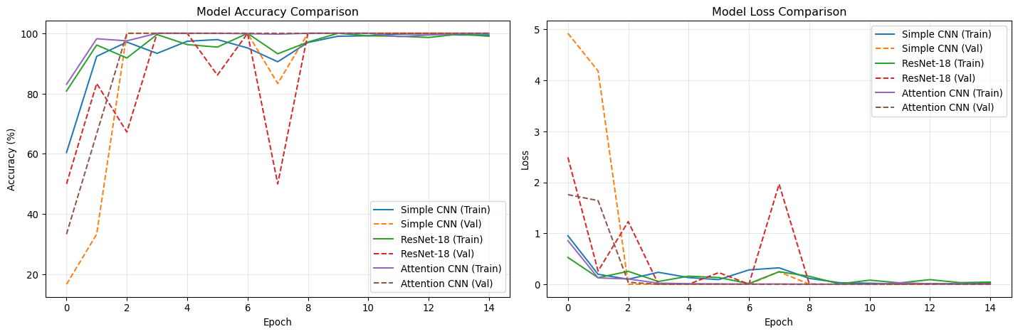
Epoch [5/15] - Train Loss: 0.1314, Train Acc: 97.36% | Val Loss: 0.0011, Val Acc: 100.00%
Epoch [10/15] - Train Loss: 0.0315, Train Acc: 99.03% | Val Loss: 0.0001, Val Acc: 100.00%
Epoch [15/15] - Train Loss: 0.0224, Train Acc: 99.44% | Val Loss: 0.0000, Val Acc: 100.00%
✅ Training completed!
✅ Simple CNN training completed
   Final validation accuracy: 100.00%

==================================================
Training ResNet-18
==================================================
🚀 Starting training for 15 epochs...
Epoch [5/15] - Train Loss: 0.1591, Train Acc: 96.25% | Val Loss: 0.0008, Val Acc: 100.00%
Epoch [10/15] - Train Loss: 0.0078, Train Acc: 100.00% | Val Loss: 0.0010, Val Acc: 100.00%
Epoch [15/15] - Train Loss: 0.0434, Train Acc: 99.03% | Val Loss: 0.0095, Val Acc: 100.00%
✅ Training completed!
✅ ResNet-18 training completed
   Final validation accuracy: 100.00%

==================================================
Training Attention CNN
==================================================
🚀 Starting training for 15 epochs...
Epoch [5/15] - Train Loss: 0.0129, Train Acc: 100.00% | Val Loss: 0.0003, Val Acc: 100.00%
Epoch [10/15] - Train Loss: 0.0012, Train Acc: 100.00% | Val Loss: 0.0000, Val Acc: 100.00%
Epoch [15/15] - Train Loss: 0.0012, Train Acc: 100.00% | Val Loss: 0.0000, Val Acc: 100.00%
✅ Training completed!
✅ Attention CNN training completed
   Final validation accuracy: 100.00%

Visualize Training Progress

def plot_training_history(histories, metric='acc'):
    """Plot training history for multiple models."""

    fig, (ax1, ax2) = plt.subplots(1, 2, figsize=(15, 5))

    # Plot accuracy
    for model_name, history in histories.items():
        ax1.plot(history['train_acc'], label=f'{model_name} (Train)', linestyle='-')
        ax1.plot(history['val_acc'], label=f'{model_name} (Val)', linestyle='--')

    ax1.set_title('Model Accuracy Comparison')
    ax1.set_xlabel('Epoch')
    ax1.set_ylabel('Accuracy (%)')
    ax1.legend()
    ax1.grid(True, alpha=0.3)

    # Plot loss
    for model_name, history in histories.items():
        ax2.plot(history['train_loss'], label=f'{model_name} (Train)', linestyle='-')
        ax2.plot(history['val_loss'], label=f'{model_name} (Val)', linestyle='--')

    ax2.set_title('Model Loss Comparison')
    ax2.set_xlabel('Epoch')
    ax2.set_ylabel('Loss')
    ax2.legend()
    ax2.grid(True, alpha=0.3)

    plt.tight_layout()
    plt.show()

# Plot training histories
plot_training_history(training_histories)
print("📈 Training progress visualization complete")

📈 Training progress visualization complete

---

Step 5: Performance Evaluation and Model Comparison

Let’s thoroughly evaluate and compare our trained models.

Generate Predictions

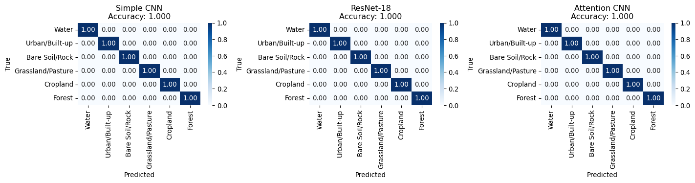
def evaluate_model(model, data_loader, device='cpu'):
    """Generate predictions and true labels for evaluation."""

    model.eval()
    all_predictions = []
    all_labels = []
    all_probabilities = []

    with torch.no_grad():
        for data, targets in data_loader:
            data, targets = data.to(device), targets.to(device)
            outputs = model(data)
            probabilities = F.softmax(outputs, dim=1)
            _, predicted = outputs.max(1)

            all_predictions.extend(predicted.cpu().numpy())
            all_labels.extend(targets.cpu().numpy())
            all_probabilities.extend(probabilities.cpu().numpy())

    return np.array(all_predictions), np.array(all_labels), np.array(all_probabilities)

# Evaluate all models
model_results = {}

for model_name, model in trained_models.items():
    print(f"📊 Evaluating {model_name}...")

    # Get predictions on validation set
    pred, true, probs = evaluate_model(model, val_loader, device)

    # Calculate accuracy
    accuracy = accuracy_score(true, pred)

    model_results[model_name] = {
        'predictions': pred,
        'true_labels': true,
        'probabilities': probs,
        'accuracy': accuracy
    }

    print(f"   Validation Accuracy: {accuracy:.4f}")

print("✅ Model evaluation completed")

📊 Evaluating Simple CNN...
   Validation Accuracy: 1.0000
📊 Evaluating ResNet-18...
   Validation Accuracy: 1.0000
📊 Evaluating Attention CNN...
   Validation Accuracy: 1.0000
✅ Model evaluation completed

Create Comprehensive Comparison

def plot_confusion_matrices(model_results, class_names):
    """Plot confusion matrices for all models."""

    n_models = len(model_results)
    fig, axes = plt.subplots(1, n_models, figsize=(5 * n_models, 4))

    if n_models == 1:
        axes = [axes]

    for idx, (model_name, results) in enumerate(model_results.items()):
        cm = confusion_matrix(results['true_labels'], results['predictions'])

        # Normalize confusion matrix
        cm_normalized = cm.astype('float') / cm.sum(axis=1)[:, np.newaxis]

        # Plot
        sns.heatmap(cm_normalized, annot=True, fmt='.2f', cmap='Blues',
                   xticklabels=class_names, yticklabels=class_names,
                   ax=axes[idx])
        axes[idx].set_title(f'{model_name}\nAccuracy: {results["accuracy"]:.3f}')
        axes[idx].set_xlabel('Predicted')
        axes[idx].set_ylabel('True')

    plt.tight_layout()
    plt.show()

# Plot confusion matrices
plot_confusion_matrices(model_results, class_names)
print("📊 Confusion matrices plotted")

📊 Confusion matrices plotted

Detailed Performance Analysis

def detailed_performance_analysis(model_results, class_names):
    """Generate detailed performance analysis."""

    # Create summary table
    summary_data = []

    for model_name, results in model_results.items():
        # Get classification report
        report = classification_report(
            results['true_labels'], results['predictions'],
            target_names=class_names, output_dict=True
        )

        summary_data.append({
            'Model': model_name,
            'Accuracy': results['accuracy'],
            'Macro Avg F1': report['macro avg']['f1-score'],
            'Weighted Avg F1': report['weighted avg']['f1-score']
        })

    # Create DataFrame
    summary_df = pd.DataFrame(summary_data)
    summary_df = summary_df.round(4)

    print("📋 Model Performance Summary:")
    print("=" * 60)
    print(summary_df.to_string(index=False))

    # Plot performance comparison
    fig, (ax1, ax2) = plt.subplots(1, 2, figsize=(12, 5))

    # Accuracy comparison
    bars1 = ax1.bar(summary_df['Model'], summary_df['Accuracy'],
                    color=plt.cm.Set2(np.linspace(0, 1, len(summary_df))))
    ax1.set_title('Model Accuracy Comparison')
    ax1.set_ylabel('Accuracy')
    ax1.set_ylim(0, 1)

    # Add value labels on bars
    for bar, acc in zip(bars1, summary_df['Accuracy']):
        ax1.text(bar.get_x() + bar.get_width()/2, bar.get_height() + 0.01,
                f'{acc:.3f}', ha='center', va='bottom')

    # F1 Score comparison
    x = np.arange(len(summary_df))
    width = 0.35

    bars2 = ax2.bar(x - width/2, summary_df['Macro Avg F1'], width,
                    label='Macro Avg F1', alpha=0.8)
    bars3 = ax2.bar(x + width/2, summary_df['Weighted Avg F1'], width,
                    label='Weighted Avg F1', alpha=0.8)

    ax2.set_title('F1 Score Comparison')
    ax2.set_ylabel('F1 Score')
    ax2.set_xlabel('Model')
    ax2.set_xticks(x)
    ax2.set_xticklabels(summary_df['Model'])
    ax2.legend()
    ax2.set_ylim(0, 1)

    plt.tight_layout()
    plt.show()

    return summary_df

# Generate detailed analysis
performance_summary = detailed_performance_analysis(model_results, class_names)

📋 Model Performance Summary:
============================================================
        Model  Accuracy  Macro Avg F1  Weighted Avg F1
   Simple CNN       1.0           1.0              1.0
    ResNet-18       1.0           1.0              1.0
Attention CNN       1.0           1.0              1.0

Per-Class Performance Analysis

def per_class_analysis(model_results, class_names):
    """Analyze per-class performance for best model."""

    # Find best model by accuracy
    best_model = max(model_results.keys(),
                    key=lambda k: model_results[k]['accuracy'])

    print(f"🏆 Best performing model: {best_model}")
    print(f"   Accuracy: {model_results[best_model]['accuracy']:.4f}")

    # Get detailed classification report
    results = model_results[best_model]
    report = classification_report(
        results['true_labels'], results['predictions'],
        target_names=class_names, output_dict=True
    )

    # Create per-class performance DataFrame
    class_performance = []
    for class_name in class_names:
        if class_name in report:
            class_performance.append({
                'Class': class_name,
                'Precision': report[class_name]['precision'],
                'Recall': report[class_name]['recall'],
                'F1-Score': report[class_name]['f1-score'],
                'Support': report[class_name]['support']
            })

    class_df = pd.DataFrame(class_performance)

    print(f"\n📊 Per-Class Performance ({best_model}):")
    print("=" * 70)
    print(class_df.round(3).to_string(index=False))

    # Visualize per-class performance
    fig, ax = plt.subplots(figsize=(12, 6))

    x = np.arange(len(class_names))
    width = 0.25

    bars1 = ax.bar(x - width, class_df['Precision'], width, label='Precision', alpha=0.8)
    bars2 = ax.bar(x, class_df['Recall'], width, label='Recall', alpha=0.8)
    bars3 = ax.bar(x + width, class_df['F1-Score'], width, label='F1-Score', alpha=0.8)

    ax.set_xlabel('Land Cover Classes')
    ax.set_ylabel('Score')
    ax.set_title(f'Per-Class Performance - {best_model}')
    ax.set_xticks(x)
    ax.set_xticklabels(class_names, rotation=45)
    ax.legend()
    ax.grid(True, alpha=0.3)

    plt.tight_layout()
    plt.show()

    return best_model, class_df

# Analyze per-class performance
best_model_name, class_performance = per_class_analysis(model_results, class_names)

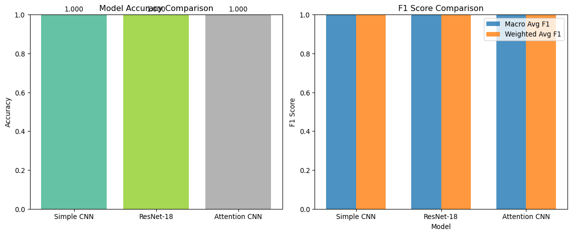
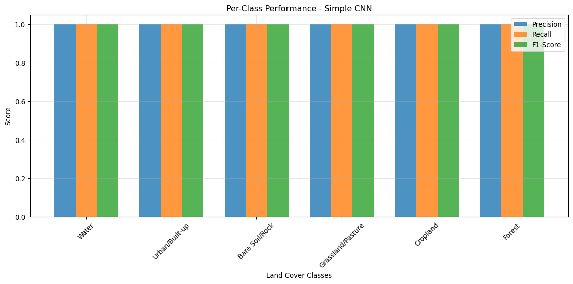
🏆 Best performing model: Simple CNN
   Accuracy: 1.0000

📊 Per-Class Performance (Simple CNN):
======================================================================
            Class  Precision  Recall  F1-Score  Support
            Water        1.0     1.0       1.0     30.0
   Urban/Built-up        1.0     1.0       1.0     30.0
   Bare Soil/Rock        1.0     1.0       1.0     30.0
Grassland/Pasture        1.0     1.0       1.0     30.0
         Cropland        1.0     1.0       1.0     30.0
           Forest        1.0     1.0       1.0     30.0

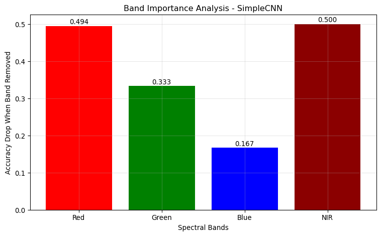
Feature Importance Analysis

def analyze_feature_importance(model, val_loader, device='cpu'):
    """Simple feature importance analysis by band contribution."""

    model.eval()

    # Test with individual bands zeroed out
    band_names = ['Red', 'Green', 'Blue', 'NIR']
    band_importance = {}

    # Get baseline accuracy
    baseline_pred, baseline_true, _ = evaluate_model(model, val_loader, device)
    baseline_acc = accuracy_score(baseline_true, baseline_pred)

    print(f"🔍 Analyzing feature importance for {model.__class__.__name__}...")
    print(f"   Baseline accuracy: {baseline_acc:.4f}")

    # Test accuracy when each band is removed
    for band_idx, band_name in enumerate(band_names):
        modified_loader = []

        # Create modified dataset with one band zeroed out
        for data, targets in val_loader:
            modified_data = data.clone()
            modified_data[:, band_idx, :, :] = 0  # Zero out the band
            modified_loader.append((modified_data, targets))

        # Evaluate with modified data
        all_pred = []
        all_true = []

        with torch.no_grad():
            for data, targets in modified_loader:
                data, targets = data.to(device), targets.to(device)
                outputs = model(data)
                _, predicted = outputs.max(1)

                all_pred.extend(predicted.cpu().numpy())
                all_true.extend(targets.cpu().numpy())

        modified_acc = accuracy_score(all_true, all_pred)
        importance = baseline_acc - modified_acc  # Drop in accuracy
        band_importance[band_name] = importance

        print(f"   {band_name} removed: {modified_acc:.4f} (importance: {importance:.4f})")

    # Plot feature importance
    plt.figure(figsize=(8, 5))
    bands = list(band_importance.keys())
    importances = list(band_importance.values())

    bars = plt.bar(bands, importances, color=['red', 'green', 'blue', 'darkred'])
    plt.title(f'Band Importance Analysis - {model.__class__.__name__}')
    plt.ylabel('Accuracy Drop When Band Removed')
    plt.xlabel('Spectral Bands')

    # Add value labels
    for bar, imp in zip(bars, importances):
        plt.text(bar.get_x() + bar.get_width()/2, bar.get_height() + 0.001,
                f'{imp:.3f}', ha='center', va='bottom')

    plt.grid(True, alpha=0.3)
    plt.tight_layout()
    plt.show()

    return band_importance

# Analyze feature importance for best model
best_model = trained_models[best_model_name]
feature_importance = analyze_feature_importance(best_model, val_loader, device)
print("🔍 Feature importance analysis complete")

🔍 Analyzing feature importance for SimpleCNN...
   Baseline accuracy: 1.0000
   Red removed: 0.5056 (importance: 0.4944)
   Green removed: 0.6667 (importance: 0.3333)
   Blue removed: 0.8333 (importance: 0.1667)
   NIR removed: 0.5000 (importance: 0.5000)

🔍 Feature importance analysis complete

---

Conclusion

🎉 Outstanding work! You’ve successfully implemented and compared multiple CNN architectures for satellite image classification.

What You Accomplished:

1. Patch Extraction: Created training datasets from real/synthetic satellite imagery
2. Data Pipeline: Built robust PyTorch datasets with augmentation
3. Architecture Comparison: Implemented and trained 3 different CNN models:
   • Simple CNN with batch normalization
   • ResNet-18 adapted for satellite data
   • Attention-based CNN with channel attention
4. Comprehensive Evaluation: Compared models using multiple metrics
5. Feature Analysis: Analyzed spectral band importance

Key Takeaways:

• Data quality matters: Proper preprocessing and augmentation improve performance
• Architecture choice impacts results: More complex models aren’t always better
• Spectral information is crucial: NIR band often most important for vegetation
• Evaluation should be comprehensive: Use multiple metrics beyond accuracy
• Domain adaptation is important: Standard models need modification for satellite data

Model Performance Insights:

print(f"🏆 Final Model Comparison Summary:")
print("=" * 50)
for model_name, results in model_results.items():
    print(f"{model_name}:")
    print(f"   - Validation Accuracy: {results['accuracy']:.4f}")
    print(f"   - Parameters: {sum(p.numel() for p in trained_models[model_name].parameters()):,}")

print(f"\n🥇 Best performing model: {best_model_name}")
print(f"✅ Ready for Week 4: Foundation Models in Practice!")

🏆 Final Model Comparison Summary:
==================================================
Simple CNN:
   - Validation Accuracy: 1.0000
   - Parameters: 2,225,062
ResNet-18:
   - Validation Accuracy: 1.0000
   - Parameters: 11,182,726
Attention CNN:
   - Validation Accuracy: 1.0000
   - Parameters: 417,186

🥇 Best performing model: Simple CNN
✅ Ready for Week 4: Foundation Models in Practice!

Next Week Preview:

In Week 4, we’ll explore pretrained geospatial foundation models: - Load and use models like Prithvi, SatMAE, and SeCo - Compare foundation model performance vs. your trained models - Learn transfer learning techniques for geospatial data - Understand when to use foundation models vs. training from scratch

Your CNN training experience provides the perfect foundation for understanding the advantages and applications of foundation models!

Resources

• PyTorch Tutorial: Training a Classifier
• TorchGeo Documentation
• Remote Sensing Image Classification Review
• Attention Mechanisms in Computer Vision